
Probability and Statistics for Engineering and the Sciences 8th Edition Chapter 3 Discrete Random Variables and Probability Distributions
Page 113 Problem 1 Answer
Given –
| y | 0 | 1 | 2 | 3 |
| P(y) | 0.6 | 0.25 | 0.1 | 0.05 |
We will find E(Y).
We will use the formula E(Y)=∑yp(y).
Applying the formula of expectation for the given data, we get:
E(Y)=∑yp(y)
E(Y) =(0×0.6)+(1×0.25)+(2×0.1)+(3×0.05)
E(Y) =0+0.25+0.2+0.15
E(Y) =0.6
We obtain: E(Y)=0.6
Page 113 Problem 2 Answer
Given –
| y | 0 | 1 | 2 | x |
| P(y) | 0.6 | 0.25 | 0.1 | 0.05 |
We will calculate E(100Y2)
We note from previous part that E(Y2)=57.25.
We have:
E(Y2)=57.25
E(100Y2)=100E(Y2)
E(100Y2) =100⋅57.25
E(100Y2) =5725
We obtain : E(100Y2)=5725
Probability And Statistics For Engineering 8th Edition Solutions Exercise 3.3 Page 113 Problem 3 Answer
We are given that P(X=0)=1−p
P(X=1)=p
We will find E(X2).We will useE(X2)=∑x2p(x).
Applying the formula, we get:
E(X2)=∑x2p(x)=[02×p(0)]+[12×p(1)]=[02×(1−p)]+[12×p]=p
We obtain: E(X2)=p
Page 113 Problem 4 Answer
Given -P(X:0)=1−p
P(X:1)=p
We will show that V(X)=p(1−p).
We know the formula V(X)=E(X2)−[E(x)]2.
We know that V (X)
E(X)= E(X − [E(x)]2)2
= ∑xp(x)
Now, = [0 × p(0)] + [1 × p(1)]
= [0 × (1 − p)] + [1 × p]
= p
Putting these values in the above formula, we get:
V (X) = E(X − [E(x)]2)2
V (X) = p − [p]2
V (X) = p − p2
V (X) = p(1 − p)
We showed that V(X)=p(1−p).
Page 113 Problem 5 Answer
Given: If X be the Bernoulli random variable with P(X:0)=1−p
P(X:1)=p
We will find E(X79)
Using the definition, we obtain:
E(X79)=[079×p(0)]+[179×p(1)]=[079×(1−p)]+[179×p]=p
We obtain the value:
E(X79)=p
Chapter 3 Exercise 3.3 Discrete Random Variables Solved Examples Page 113 Problem 6 Answer
Given – The data:
x 1 2 3 4 5 6
p(x) 1/15 2/15 3/15 4/15 5/15 6/15
We also know that owner bought copy for $2.00 and sells it for$4.00.
We will justify whether to buy 3 or 4 copies per week. We will find E(X),
If n=3, we note that owner bought 3copies.
E(x) is the expected value it is given by sum of the products ofx
value with p(x).
Hence, after x=3 multiply p(x) with 3.
Using E(x)=x=1
∑ x⋅p(x) ∞, we get L E(x)=1(1/15)+2(1/15)+3(1/15)+3(4/15)+3(3/15)+3(2/15)
=41/15
=2.733
The cost of 3 copies is given as 3(2)=6
We conclude that the owner sells those 3 copies at 4 each.
We suppose the net revenue, R=4(x)−6.
IT is in the form of W=a(x)+b.
Using the formula for expectation, we get:
E(aX+b)=a(E(x))+b
Here E(x)=E[4(x)−6] here a=4 ,b=6
Hence E(W)=4
E(x)−6
Using its value from the previous step , we get:
E(x)=41/15
E(x)= 2.733
Thus,E(W)=4(41/15)−6
≈4.933
Now, we will suppose n=4.
let us assume that owner bought 4 copies .
We note the formula:
E(x)=n=0
∑ x⋅p(x)
∞ So , the expectation is:
E(x)=n=0
∑ x⋅p(x) ∞
E(x)=1(1/15)+2⋅(1/15)+3(1/15)+4(4/15)+4(3/15)+4(2/15)
E(x)= 50/15
≈3.33
The cost of 4 copies is given as 4(2.00)=8.00.
Hence, the owner sells those 4 copies at 8 each.
We know that the net revenue is R=4(x)−8.
It is in the form of W=a(x)+b.
Therefore, the expected value of this can be calculated as:
E(x)=E[4(x)−8]
Here a=4 b=8
Hence E(W)=4
E(x)−8
Using the previous step, we get:
E(x)=10/3=3.733 approx
Hence E(W)=4(10/3)−8=5.33 3approx.
If owner buys 3 copies he will get net revenue of 4.933.
If he if owner buys 4 copies he will get net revenue of 5.333
Clearly, it is better to buy 4 copies.
Chapter 3 Exercise 3.3 Study Guide Probability And Statistics Page 114 Problem 7 Answer
Given – A random variable x and x is the random variable for both the batches. so we need to calculate both mean and variance of x .
After computing mean and variance we also need to compute expected number of pounds after the next customer product is shipped and variance of pound left
We also have that a company has 100 lb of certain chemical in stock The customer orders in 5 lb batches do we are left with100−5X lb’s in total
We will find mean and variance for this.
Using the definition, we get:
E(x)=x=1
∑ xp(x) ∞
=1(0.2)+2(0.4)+3(0.3)+4(0.1)
=2.3
Also, the variance is:
V(x)E(x2)=[E(x2)−E(x)2]
=1(0.2)+2(0.4)+3(0.3)+4(0.1)
=6.1
Putting the obtained values, we get:
V(x)=[E(x2)−[E(x)]2]
=6.1−(2.3)2
=0.81
We observe that 100−5X is in the form of a(x)+b
So, applying the rule:
E(aX+b)=a(E(x))+b=(−5)E(x)+100
Here a=−5
b=100
So −5(E(x))+100=−5(2.3)+100
=88.5.
We also have the rule V(ax)=a2
v(x) for constant v(x) is zero.
Hence,
V(100−5x)=(−5)2
V(x)=20.25
We obtain:
E(x)=2.3
V(x)=0.81
E(100−5X)=88.5
V(100−5X)=20.25
Page 113 Problem 8 Answer
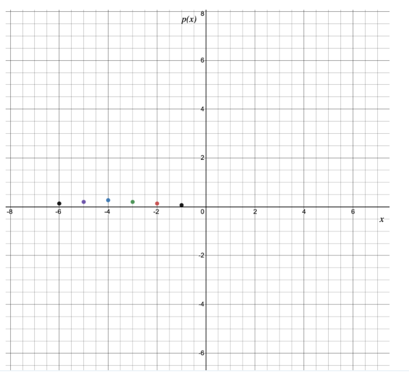
We will plot a graph for pm f(x), We are given x and p(x) values.
For the data given , we obtain the graph as:
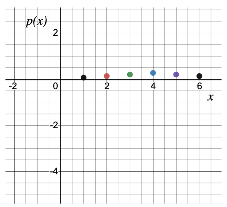
We note that for the given x values and p(x) values, in order to plot graph for negative values of x we will multiply x with−1.
Clearly, the spread of both these graphs is same.
Therefore, we can say that V(X)=V(−X).
Using the spread in graphs, we showed that V (X) = V (−X).
Page 114 Problem 9 Answer
Using the formula we can prove that V(X)=V(−X)
We note that the variance is given as V(aX+b)=a{2}
(v(x)) for constant V(x) is zero
According to the formula V(aX+b)=a{2}
V(x) for constant V(x) is zero
Here, inV(−X)
we have: a=−1
b=0
Now, using the formula we can prove that V(x)=V(−x) , It is in the form of V(aX+b) here a=−1 and b=0
ThusV(−x)=(−1){2} V(x).
It is equal to V(x).
Hence,V(x)=V(−x)
With the help of proposition involving V(aX+b), we showed that V(x)=V(−x).
Discrete Random Variables Examples From Exercise 3.3 Engineering And Sciences Page 114 Problem 10 Answer
We will prove that V(aX+b)=a2⋅σX2
We note that:
h(X)=aX+bV(aX+b)
=a2⋅σy2
We also note that
h(X)=aX+bE[h(X)]
=aμ+b
Here μ=E(X).
The variance of a X+b is given by:V(aX+b)=[E(aX+b)2−(E(aX+b))2]
Using the given data, we obtain:
∞
V (aX + b) = ∑ (x − μ)2 p(x)V (aX + b)
∀
∞
=∑ [E ( (aX + b)2) − (E(aX + b))2]
∀
V (aX + b) = [aX − aμ] ⋅ p(x)
We see that a is constant so taking a out of the summation it becomes a2
Thus, V(aX+b)=a2
∀
∑ (x−(E(x))2)⋅p(x)
∞
V(aX+b)=a{2}
V(x) We showed that V(aX+b)=a2 V(X).
Page 114 Problem 11 Answer
Given -a≤X≤b
We need to show that a≤E(X)≤b.
We will use: E(X)=μx
μx=∑x∈S x⋅p(x)
Multiplying p(x) in the given inequality, we get:
a≤x≤b
So, a⋅p(x)≤x⋅p(x)≤b⋅p(x)
For all x∈S. This now implies that for the sum over all x∈S, the given inequality is satisfied.
x∈S
∑ a⋅p(x)≤x∈S
∑ x⋅p(x)≤x∈S
∑ b⋅p(x)
We obtain:
x∈S
∑ a⋅p(x) x∈S
∑ b⋅p(x) =a⋅x∈S
∑ p(x) =a⋅1=a;
=b⋅x∈S
∑ p(x) =b⋅1=b;
So, the sum over all x∈S of pmf p(x) is 1
We have that E(X)=x∈S
∑ x⋅p(x)
Hence, using the data obtained, we get: a≤E(X)≤b
Fora≤X≤b we showed that a≤E(X)≤b.