Introduction to Probability and Statistics Principles and Applications Chapter 1 Introduction to Probability and Counting Exercises
Introduction to Probability and Statistics Chapter 1 exercises solutions Page 14 Exercise 1 Problem 1
According to the question, A government study defines a “group 1” nuclear accident to be one involving severe core damage, melting of uranium fuel, essential failure of all safety systems, and a major breach of the reactor’s containment resulting in a large release of radioactivity into the atmosphere.
In1982, officials at Nuclear Regulatory commission estimated the probability of such an accident occurring in the United States before the year 2000 to be.02.
We need to tell which approach to probability is used to determine the value.
According to data given in the question it has dangerous consequences, this experiment definitely isn’t repeatable.
So, officials at the Nuclear Regulatory Commission estimated the given probability by using Classical Method.
Officials at Nuclear Regulatory commission estimated the probability of such an accident occurring in the United States before the year 2000 to be.02 by using Classical Method.
J. Susan Milton Probability And Counting Chapter 1 Answers Page 14 Exercise 2 Problem 2
According to the question, Hemophilia is a sex-linked hereditary blood defect of the males characterized by delayed clotting of the blood which makes it difficult to control bleeding even in the case of a minor injury.
When a woman is carrier of classical hemophilia there is 50%chance that a male child will inherit the disease.
We need to answer what will be the probability that the carrier gives birth to two sons and the approach we used to find the probability.
Read and Learn More J Susan Milton Introduction To Probability And Statistics Solutions
According to data given in the question, we have four possible outcomes for sons to have or not to have disease
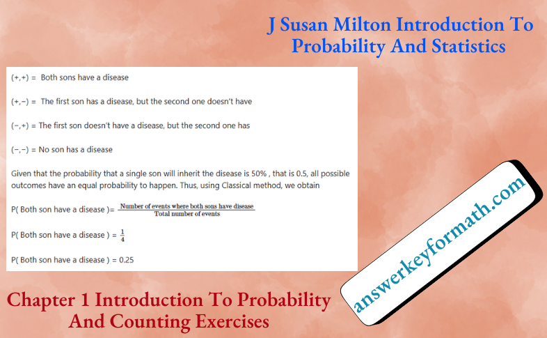
The probability that the carrier gives birth to two sons is 0.25 and the approach we used to find the probability is Classical Method.
J Susan Milton Introduction To Probability And Statistics Chapter 1 Page 14 Exercise 3 Problem 3
According to the question, The probability of having a fatal accident in the work place is assessed using the fatal accident frequency rate (FAFR).
This rate is defined by
FAFR = Number of fatalities per1000workers during a working lifetime.
We need to find the approach to probability of an individual having fatal accident while at work.
Also, Find the approximate probability that a coal miner will suffer a fatal injury. Coal mining industry and is taken into account when computing the industry-wide FAFR of 4.
We need to explain how the rate could be so low while at least some of the components used in its computation are high.
Given that FAFR = Number of fatalities per1000workers during a working lifetime.
Hence we use the relative frequency approach to approximate the given probability
Given that FAFR for coal mining occupation is 12
We use the relative frequency approach, hence we conclude that the probability that a coal miner will suffer a fatal injury is.
⇒ \(\frac{12}{1000}\)
= 0.012
The overall industry FAFR is equal to 4 because for a large number of occupations, FAFR is very low because those occupations are not dangerous and risky for human life.
The probability approach we used is relative frequency approach. The probability that a coal miner will suffer a fatal injury is 0.012. Coal mining industry and is taken into account when computing the industry-wide FAFR of 4, that is very low because those occupations are not dangerous and risky for human life.
Solutions To Probability And Counting Exercises Chapter 1 Susan Milton Page 15 Exercise 4 Problem 4
Questions explains that in ballistics studies conducted during World War II, it was found that inground-to-ground firing, artillery shells tended to fall in an elliptical pattern such as given in the question.
The probability that a shell would fall in the inner ellipse is 0.50 ; the probability that it would fall in the outer ellipse is 0.95.
A firing is considered to be a success (s)if the shell falls within the inner ellipse; otherwise, it is failure (f).
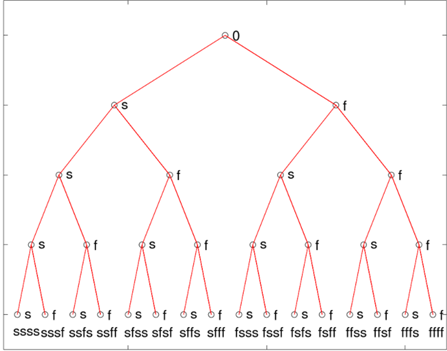
We need to construct a tree to represent the firing of four shells in succession.
For each of the four shells, we have two possible outcomes (given shell falls within inner ellipse) or f (given shell doesn’t fall within inner ellipse).
Hence the tree diagram that represent the firing of four shells in succession as follows
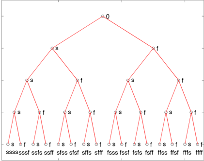
The tree diagram that represent the firing of four shells in succession as follows
J Susan Milton Introduction To Probability And Statistics Chapter 1 Page 15 Exercise 5 Problem 5
Questions explains that in ballistics studies conducted during World War II, it was found that inground-to ground firing, artillery shells tended to fall in an elliptical pattern such as given in the question.
The probability that a shell would fall in the inner ellipse is 0.50 ; the probability that it would fall in the outer ellipse is 0.95.
We need to list the sample points generated by the tree.
With the help of tree diagram from Page 15 Exercise 4 Problem 4 , We conclude the sample space and sample points are:
S = {ssss,sssf,ssfs,ssff,sfss,sfsf,sfs,sfff,fsss,fssf,fsfs,fsff,ffss,ffsf,ffs,ffff}
The sample space and the sample points are: S={ssss,sssf,ssfs,ssff,sfss,sfsf,sff,sff,fsss,fssf,fsfs,fsff,ffss,ffsf,fff,ffff}
Probability and Statistics J. Susan Milton Chapter 1 solved step-by-step Page 15 Exercise 5 Problem 6
Questions explains that in ballistics studies conducted during World War II, it was found that inground-to ground firing, artillery shells tended to fall in an elliptical pattern such as given in the question.
The probability that a shell would fall in the inner ellipse is 0.50 ; the probability that it would fall in the outer ellipse is 0.95.
Let Ai,i = 1,2,34 denote the event that the i−thfiring is successful. We need to list the sample points that constitute each of the events A1 ,A2,A3,A4 and check are these events mutually exclusive.
The sample points that constitute each of the events A1,A2,A3,A4 are
A1= the first firing is successfulsssss,sssf, ssfs,ssff,sfss,sfsf,sffs,sfff
A2 = The second firing is successful{ssss,sssf,ssfs,ssff,fsss,fssf,fsfs,fsff}
A3 = The third firing is successful{ssss,sssf,sfss,sfsf,fSSS,fssf,ffss,ffSf}
A4 = The fourth firing is successful{sssss, ssfs, sfss, sffs, fsss, fsfs, ffss, fffs }
A,A2,A3,A4 are not mutually exclusive events because event{ssss} is in every four events.
The sample points that constitute each of the events A1,A2 ,A3,A4 are
A1 = {ssss,sssf,ssfs,ssff,sfss,sfsf,sffs,sfff}
A2 = {ssss,sssf,ssfs,ssff,fsss,fssf,fsf,fsff
A3 = {ssss,sssf,sfss,sfsf,fsss,fssf,ffss,ffsf}
A4 = {ssss,ssfs,sfss,sffs,fsss,fsfs,ffs,fffs}
A1, A2, A3, A4 are not mutually exclusive events because event {ssss}is in every four events.
J Susan Milton Introduction To Probability And Statistics Chapter 1 Page 15 Exercise 5 Problem 7
Questions explains that in ballistics studies conducted during World War II, it was found that inground-to ground firing, artillery shells tended to fall in an elliptical pattern such as given in the question.
The probability that a shell would fall in the inner ellipse is 0.50; the probability that it would fall in the outer ellipse is 0.95.
We need to list the sample points that constitute each of these events and describe the events verbally:
A1′
A1∪A2
A1∩A2
A1∩A2∩A3∩A4
A1∩A2∩A3∩A′4
(A1∪A2∪A3∪A4)A1∩A′1
The sample points from the definition of complement, union and intersection
A1′= The first firing is not successful{fSSS,fSSf,fsfs,fsff,ffS,ffsf,fffs,fff}
A1∪A2 = The first or second firing is successful{ssss,sssf,ssfs,ssff,sfss,sfsf,sffs,sfff,fsss,fssf,fsfs,fsff}
A1∩A2 = The first and second firing is successfulsssss,sssf,ssfs,ssff}
A1∩A2∩A3∩A4 = All four firing are successful {ssss}
A1∩A2∩A3∩A′4= The first three firings are successful and the last one is not {sssf}
(A1∪A2∪A3∪A4)′ = All firings are unsuccessful {fff}
A1∩A1′= The first firing is successful and the first firing is not successful =Φ
The sample points from the definition of complement, union and intersection
A1′ = {fSSS,fssf,fsfS,fSff,fSS,ffsf,ffS,fff}
A1∪A2 = {ssss,sssf,ssfs,ssff,sfs,sfsf,sffs,sfff,fsss,fssf,fsfs,fsff}
A1∩A2 = {ssss,sssf,ssfs,ssff}
A1∩A2∩A3∩A4 = {sSSS}
A1∩A2∩A3∩A4 = {sssf}
(A1∪A2∪A3∪A4) = {ffff}
A1∩A1′ = Φ
J Susan Milton Introduction To Probability And Statistics Chapter 1 Page 15 Exercise 5 Problem 8
Questions explains that in ballistics studies conducted during World War II, it was found that inground-to ground firing, artillery shells tended to fall in an elliptical pattern such as given in the question.
The probability that a shell would fall in the inner ellipse is 0.50 ; the probability that it would fall in the outer ellipse is 0.95.
We need to find the probability of each of the events of part(d) by classical probability and why is it true.
The probability for a single shell to fall when the inner ellipse is 0.5, then he probability for a single shell to fall outside of the inner ellipse is also 0.5.From the classical method we have:
P(A) = \(\frac{\text { Number of ways } A \text { can occur }}{\text { Number of ways the experiment can proceed }}\)
Each sample point can occur in one and only one way. Also, there are 16 possible outcomes in total. So, the probability of each sample point is: 1
= \(\frac{1}{16}\)
= 0.0625
The probability of each sample point is: 0.0625
Online help for J. Susan Milton Probability Chapter 1 exercises Page 16 Exercise 6 Problem 9
We need to evaluate the expression 9!
We have expression as 9!
9! = 9 × 8 × 7 × 6 × 5 × 4 × 3 × 2 × 1
9! = 362880
The value of the expression 9! is 362880.
J Susan Milton Introduction To Probability And Statistics Chapter 1 Page 16 Exercise 6 Problem 10
We need to evaluate the expression 6!
We have expression as 6!
6! = 6 × 5 × 4 × 3 × 2 × 1
6! = 720
The value of the expression 6! is 720.
Step-by-step guide to Probability and Counting exercises Chapter 1 Milton Page 16 Exercise 6 Problem 11
We need to evaluate the expression 7P3
We have expression as 7P3
7P3 = \(\frac{7 !}{(7-3) !}\)
7P3 = \(\frac{7 !}{4 !}\)
7P3 = \(\frac{7 \times 6 \times 5 \times 4 \times 3 \times 2 \times 1}{4 \times 3 \times 2 \times 1}\)
Cancilation of (4,3,2,1)
= 7 × 6 × 5
= 210
The value of the expression 7P3 is 210.
Page 16 Exercise 6 Problem 12
We have expression as 6p2
6p2 = \(\frac{6 !}{(6-2) !}\)
6p2 = \(\frac{6 !}{4 !}\)
6p2 = \(\frac{6 \times 5 \times 4 \times 3 \times 2 \times 1}{4 \times 3 \times 2 \times 1}\)
Cancilation of (4,3,2,1)
= 6 × 5
= 30
The value of the expression 6p2 is 30.
J Susan Milton Introduction To Probability And Statistics Chapter 1 Page 16 Exercise 6 Problem 13
According to the question, in investigating the ideal Gas Law, experiment are to be run at four different pressures and three different temperatures.
We need to find the number of experimental conditions are to be studied.
The multiplication principle: Consider an experiment taking place in k stages.
Let ni denote the number of ways in which stage i can occur for i = 1,2,3,……k.
Altogether the experiment can occur in ways.
\(\prod_{i=1}^k\) ni = n1 × n2 nk
Since we have four different pressures and three different temperatures, according to the multiplication principle, we conclude that 4 × 3 = 12 experimental conditions will be studied.
12 experimental conditions are to be studied.
Exercise solutions for Chapter 1 Susan Milton Probability and Counting Page 16 Exercise 6 Problem 14
According to the question, in investigating the ideal Gas Law, experiment are to be run at four different pressures and three different temperatures.
We need to find number of experiments will be conducted on the given gas if each experiment condition is replicated five times.
The multiplication principle: Consider an experiment taking place in k stages.
Let ni denote the number of ways in which stage i can occur for i = 1,2,3,……k.
Altogether the experiment can occur in
\(\prod_{i=1}^k\) ni = n1 × n2 nk
Since, each experimental condition is repeated five times, from the multiplication principle, we conclude that 5 × 12 = 60 experimental conditions will be conducted on a given gas.
60 experimental conditions will be conducted on a given gas.
J Susan Milton Introduction To Probability And Statistics Chapter 1 Page 16 Exercise 6 Problem 15
According to the question, in investigating the ideal Gas Law, experiment is to be run at four different pressures and three different temperatures.
We need to find number of experiments will be conducted to obtain five replications on each experimental condition for each of the six different gases.
The multiplication principle: Consider an experiment taking place in k
stages.
Let ni denote the number of ways in which stage i can occur for i = 1,2,3,……k.
Altogether the experiment can occur in
\(\prod_{i=1}^k\) ni = n1 × n2 nk
Since, each of six gases, there will be 60 conducted experiments from the multiplication principle, we conclude that 6 × 60 = 360
360 experiments will be conducted to obtain five replications on each experimental condition for each of the six different gases.
Page 17 Exercise 7 Problem 16
Four artillery shells have been fired in succession, each firing is either considered as a success or a failure.
We need to use the multiplication rule to prove that the number of paths through the tree for this experiment is 16.
There are four artillery shells, k = 4
The experiment is either a success or failure for i = 1,2,3,4
Therefore n1 ,n2,n3 and n4 are equal to 2.
From the multiplication principle
\(\prod_{i=1}^4 n_i\) = 2.2.2.2.
= 16
Number of paths through the tree representing this experiment is 16.
Using the multiplication principle, the number of paths through the tree to represent the experiment which involved firing of four artillery shells is proven to be 16.
J Susan Milton Introduction To Probability And Statistics Chapter 1 Page 17 Exercise 8 Problem 17
The Apollo mission consists of five components and each component is marked as operable or inoperable but for the proper functioning of this mission all the states must be operable.
We need to indentify the number of states that are operable.
In this mission the number of components are five, k = 5.
The components are either operable or inoperable for i = 1,2,3,4,5
Hence n1 ,n2,n3,n4 and n5 is equal to 2.
Therefore, from the multiplication principle;
\(\prod_{i=1}^5 n_i\) = 2.2.2.2.2
= 32
The number of states that are operable is 32.
For the Apollo mission that consists of five components that is marked as either operable or inoperable, the number of states that are operable is found to be 32.
Page 17 Exercise 8 Problem 18
The Apollo mission consists of five components and each component is marked as operable or inoperable but for the proper functioning of this mission all the states must be operable.
We need to indentify the number of states in which LEM is inoperable.
The Apollo mission has five components in which if LEM is inoperable then the remaining states are four, k = 4.
The components are either operable or inoperable for i = 1,2,3,4
Therefore n1 ,n2 ,n3 and n4 are equal to 2.
From the multiplication principle
\(\prod_{i=1}^4 n_i\) = 2.2.2.2
= 16
The number of states in which the LEM is inoperable is 16.
For the Apollo mission that consists of five stages, the number of states when LEM Is inoperable is 16.
J Susan Milton Introduction To Probability And Statistics Chapter 1 Page 17 Exercise 8 Problem 19
The Apollo mission consists of five components and each component is marked as operable or inoperable but for the mission to be partially successful the first three components must be operable.
Therefore we need to find the number of states which represents, partially successful mission.
The mission has five components in which if the first three components are operable then the mission is considered as partially successful.
So we keep the first three components fixed and the last two components is either operable or inoperable hence according to the multiplication principle;
n4 = n5 ⇒ 2
= 2⋅2
= 4
The number of states that represent a partially successful mission
For the Apollo mission to be partially successful the first three components must be operable hence the number of states that represents a partially successful mission is 4.
Page 17 Exercise 8 Problem 20
The Apollo mission consists of five components and each component is marked as operable (o) or inoperable (i) but for the success of this mission all the states must be operable.
We need to in dentify the number of states when the mission is fully successful.
The operable state is denoted as (o) and the inoperable state is denoted as (i) For a complete successful mission all the five components must be operable and therefore the numbers of states that represent fully successful mission is ooooo.
For the Apollo mission to be fully successful the all five components must be operable hence the number of states that represents a fully successful mission is ooooo.
J Susan Milton Introduction To Probability And Statistics Chapter 1 Page 17 Exercise 9 Problem 21
Binary code consists of on (1) and off (0) values.
When each pixel is quantized to gray level using a binary code, we need to find how many gray levels can be quantized using a four bit binary code.
Four level binary code is there in which each binary digit is considered as a stage hence κ = 4
In binary system we have (0)’s and (1)’s hence n1,n2,n3 and n4 are equal to 2.
From the multiplication principle
\(\prod_{i=1}^4 n_i\) = 2.2.2.2
The number of gray levels that are quantized using four bit binary system is 16.
The number of gray levels that are quantized using four bit binary system is 16.
Page 17 Exercise 9 Problem 22
Binary code consists of on (1) and off (0) values.
We need to find the number of bits required to code a pixel that is quantized to 32 grey levels
The number of bits required is the number of stages which is equal to k.
Since there are two possibilities0and 1 we have, 2⋅2⋅2⋅…⋅nk = 32
2k = 32
k = 5 since (25 = 32)
Therefore the number of bits of binary code that is required to code a pixel that is quantized to 32 grey levels is 5.
The number of bits of binary code that is required to code a pixel that is quantized to 32 grey levels is 5.
J Susan Milton Introduction To Probability And Statistics Chapter 1 Page 17 Exercise 10 Problem 23
We know that nCr= \(\left(\begin{array}{l}n \\r\end{array}\right)\) = \(\frac{n !}{r !(n-r) !}\) , hence we have to prove nCr = nCn-r
We know that nCr = \(\left(\begin{array}{l}n \\r \end{array}\right) \Rightarrow \frac{n !}{r !(n-r) !}\)
So , Cn-r = \(=\left(\begin{array}{l}n \\n-r\end{array}\right) \Rightarrow \frac{n !}{(n-r) !(n-(n-r)) !}\)
Cn-r = \(\frac{n !}{r !(n-r) !} \Rightarrow{ }_n C_r\)
Hence nCr = nCn-r
Since nCr=\(\left(\begin{array}{l}n \\r\end{array}\right) \Rightarrow \frac{n !}{r !(n-r) !}\) and also Cn-r =\(\left(\begin{array}{l}n \\n-r\end{array}\right)\) \(\Rightarrow \frac{n !}{(n-r) !(n-(n-r)) !}\) , we prove that nCr = nCn-r.
Page 17 Exercise 11 Problem 24
Given five compilers, pair wise comparisons are done hence we need to find the combinations of these five compilers selected two at a time.
The number of compilers is five, n = 5
Two are compared, r = 2
Substituting in the equation nCr = \(\left(\begin{array}{l}n \\r\end{array}\right)\) \(\Rightarrow \frac{n !}{r !(n-r) !}\)
5C2 = \(\left(\begin{array}{l}5 \\2\end{array}\right) \Rightarrow \frac{5 !}{2 !(5-2) !}\)
5C2 = \(\frac{5 \cdot 4 \cdot 3 \cdot 2 \cdot 1}{2 \cdot 1(3 \cdot 2 \cdot 1)}\)
5C2 = \(\frac{20}{2}\)
5C2 = 10
The number of pair wise comparisons made are 10.
Given five compilers, the number of pair wise comparisons made are 10.
J Susan Milton Introduction To Probability And Statistics Chapter 1 Page 17 Exercise 12 Problem 25
We need to use the formula nCr = \(\frac{n !}{r !(n-r) !}\)
Where
n = 103 Is the pool of qualified applicants
r = 22 Is number of applications to select.
We need to find nCr = \(\frac{n !}{r !(n-r) !}\)
Substituting values
nCr = \(\frac{n !}{r !(n-r) !}\)
Substituting values
nCr ⇒ \(\frac{103 !}{22 !(81) !}\)
nCr ⇒ 1.51978828 × 10²²
The number of ways 22 applications can be selected from a pool of 103 applications is 1.51978828 × 10²².
Page 17 Exercise 12 Problem 26
We need to use the formula = \(\frac{n !}{r !(n-r) !}\)
Considering that you are one of the applicants, we need to find the number of pools you will be included it.
Thus, of the 22 people, you are one of them and the other 21 people will be chosen from a pool of 102
Where
n = 102 is the pool of qualified applicants
r = 21 Is number of applications to select.
Substituting values
nCr = \(\frac{n !}{r !(n-r) !}\)
nCr ⇒ \(\frac{102 !}{21 !(81) !}\)
nCr ⇒ 3.25 × 10 21
The number of sub-groups you will be included in is 3.25 × 10 21.
J Susan Milton Introduction To Probability And Statistics Chapter 1 Page 17 Exercise 12 Problem 27
We need to find the probability of being selected considering all candidates are equal.
The number of times you will be in the pool of selected applicant is 3.25 × 10 22.
The total number of ways pools can be formed is 1.52 × 10 22
We need to find the probability of getting selected.
Find the probability of being selected
P(A) = \(\frac{A}{B}\)
⇒ \(\frac{3.25 \times 10^{21}}{1.52 \times 10^{22}}\)
⇒ 0.21
The probability of getting selected from a pool of 103 applicants is 0.21.
J Susan Milton Introduction To Probability And Statistics Chapter 1 Page 18 Exercise 13 Problem 28
There are 128 – bit messages.
Each bit can be either correct or incorrect.
Hence, the total number of possible messages are 2 218
We need to find the number of cases where only two of these bits are wrong and the rest are correct.
For this we look at number of ways two bits can be selected of theone-twenty-eight.
Using that, we shall find the probability.
Find the number of events satisfying our condition
nCr = \(\frac{n !}{r !(n-r) !}\)
128 C2 = \(\frac{128 !}{2 !(128-2) !}\)
Find the probability
The parobability of two of the bits being wrong
⇒ \(\frac{2-b i t s}{\text { Total }}\)
⇒ \(\frac{\frac{128 !}{2 !(128-2) !}}{2^{128}}\)
⇒ 2.39 10– 35
⇒ \(\frac{127 \times 64}{2^{128}}\)
The probability of only two of the bits being wrong is 2.39 × 10– 35
J Susan Milton Introduction To Probability And Statistics Chapter 1 Page 18 Exercise 13 Problem 29
There are \(\frac{n !}{n_{1} ! \times n_{2} ! \ldots n_{k} !}\) experiments with 4 different temperatures, each three times.
So, comparing with
n = n1 + n2 +…+ nk
12 = 3 + 3 + 3 + 3
We need to find the number of ways the experiment can be conducted.\(\frac{n !}{n_{1} ! \times n_{2} ! \ldots n_{k} !}\)
Substituting into \(\frac{n !}{n_{1} ! \times n_{2} ! \ldots n_{k} !}\)
⇒ \(\frac{12 !}{3 ! \times 3 ! \times 3 ! \times 3 !}\)
⇒ 369600
The number of ways the experiment can be conducted is 369600.
J Susan Milton Introduction To Probability And Statistics Chapter 1 Page 18 Exercise 13 Problem 30
We need to prove that \(\left(\begin{array}{c}
n \\
n_1
\end{array}\right)\left(\begin{array}{c}
n-n_1 \\
n_2
\end{array}\right) \ldots\left(\begin{array}{c}
n-n_1-n_2 \ldots n_{k-1} \\
n_k
\end{array}\right)\) = \(\frac{n !}{n_{1} ! \times n_{2} ! \ldots n_{k} !}\)
⇒ \(\frac{n !}{n_{1} !\left(n-n_1\right) !} \times \frac{\left(n-n_1\right) !}{n_{2} !\left(n-n_1-n_2\right) !} \cdots \cdot \frac{\left(n-n_1-n_2 \ldots n_{k-1}\right) !}{n_{k} !\left(n-n_1-n_2 \ldots n_k\right) !}\)
Every denominator of the numerator is cancelled out by the denominator of the previous term’s part leaving us with
\(\frac{n !}{n_{1} ! \times n_{2} ! \ldots n_{k} !\left(n-n_1-n_2 \ldots n_k\right) !}\)
⇒ \(\frac{n !}{n_{1} ! \times n_{2} ! \ldots n_{k} !(n-n) !}\)
\(\Rightarrow \frac{n !}{n_{1} ! \times n_{2} ! \ldots n_{k} !}\)
Which is the RHS
We thus proved that \(\left(\begin{array}{c}n \\n_1\end{array}\right)\left(\begin{array}{c}n-n_1 \\n_2\end{array}\right) \ldots\left(\begin{array}{c}
n-n_1-n_2 \ldots n_{k-1} \\n_k\end{array}\right)\) =\( \frac{n !}{n_{1} ! \times n_{2} ! \ldots n_{k} !\left(n-n_1-n_2 \ldots n_k\right) !}\)
J Susan Milton Introduction To Probability And Statistics Chapter 1 Page 18 Exercise 14 Problem 31
We need to find n when
\(\left(\begin{array}{l}n \\2\end{array}\right)\) = 21 , \(\left(\begin{array}{l}n \\2\end{array}\right)\) = 105
We shall use the formula \(\left(\begin{array}{l}
n \\
r
\end{array}\right)\) = \(\frac{n !}{r !(n-r) !}\)
For \(\left(\begin{array}{l}
n \\
2
\end{array}\right)\) = 21
Substituting in
\(\left(\begin{array}{l}
n \\
r
\end{array}\right)=\frac{n !}{r !(n-r) !}\)
= \(\frac{n !}{r !(n-r) !}\)
⇒ \(\frac{n !}{2 !(n-2) !}\) = 21
⇒ n(n – 1) = 21 (2)
⇒ n(n – 1) = 42
Thus we Know n = 7
For \(\left(\begin{array}{l}n \\2\end{array}\right)\) = 105
Substituting in
⇒ \(\frac{n !}{r !(n-r) !}\)
⇒ \(\frac{n !}{2 !(n-2) !}\) 105
⇒ n(n – 1) = 105(2)
⇒ n(n – 1) = (15)(14)
Thus n = 15
For \(\left(\begin{array}{l}n \\2\end{array}\right)\) = 21 , For \(\left(\begin{array}{l}n \\2\end{array}\right)\) = 105 , n = 15.
J Susan Milton Introduction To Probability And Statistics Chapter 1 Page 19 Exercise 15 Problem 32
There are 25 packages.
10 packages need to be chosen.
The number of ways this can be done is
⇒ \(\left(\begin{array}{l}25 \\10\end{array}\right)\).
Then we need to find ways to select 3 games if 5 games packages exist within the given packages.
The number of ways this can be done is
⇒ \(\left(\begin{array}{l}20 \\7\end{array}\right)\) \(\left(\begin{array}{l}5 \\3\end{array}\right)\)
Finding \(\left(\begin{array}{l}20 \\7\end{array}\right)\) , \(\left(\begin{array}{l}5 \\3\end{array}\right)\)
⇒ \(\frac{20 !}{7 !(13) !} \times \frac{5 !}{3 !(2) !}\)
= 775200
The number of ways 10 packages can be chosen is 3.27 × 10⁶. The number of ways three of these can be games is 775200.
J Susan Milton Introduction To Probability And Statistics Chapter 1 Page 19 Exercise 16 Problem 33
There are four women and six men.
We need to find the total number of ways three employees can be chosen at random.
Then we need to find the ways no women is chosen.
The ration of the two gives us the probability.
Total number of ways three employees can be chosen is
\(\left(\begin{array}{1}10\\3\end{array}\right)=\frac{10 !}{3 !(7) !}\)
⇒ 240
Number of ways no women is chosen is the number of ways three men are chosen which is
\(\left(\begin{array}{1}6 \\3\end{array}\right)=\frac{6 !}{3 !(3) !}\)
⇒ 20
Probability that no women is chosen is
⇒ \(\frac{20}{240}\)
Which is \(\frac{1}{12}\).
Probability that no women is chosen is \(\frac{1}{12}\) As the probability is very low, the occurrence of such an event is suspicious as there is a god chance that at least one woman would be chosen if randomly chosen.
J Susan Milton Introduction To Probability And Statistics Chapter 1 Page 19 Exercise 17 Problem 34
We need to use five alphabets and one digit to make the password.
Any of the twenty six alphabets and ten digits can be used.
We need to find the total number of all possible passwords.
Repeating the alphabets is allowed.
The total number of passwords that can exist are
(26)(26)(26)(26)(26)(10)
=118813760
The total number of possible passwords are 118813760.
Page 19 Exercise 17 Problem 35
We need to use five alphabets and one digit to make the password.
Any of the twenty six alphabets and ten digits can be used.
We need to find the ways three As and two Bs can be used with an even digit.
There are 5 even digits.
Repeating the alphabets is allowed.
The total number of ways three As and two Bs can be used with an even digit
⇒ \(\left(\begin{array}{1}5 \\3\end{array}\right)\) 5
⇒ \(\frac{5 !}{3 ! 2 !}\) × 5 = 50
The total number of ways three As and two Bs can be used with an even digit is 50.
Page 19 Exercise 17 Problem 36
We need to find the ways three As and two Bs can be used with an even digit.
There are 5 even digits.
The total number of ways three As and two Bs can be used with an even digit is 50.
The probability of guessing the correct password of the fifty possibilities is \(\frac{1}{50}\).
J Susan Milton Introduction To Probability And Statistics Chapter 1 Page 19 Exercise 18 Problem 37
Given: An electrical control panel has three toggle switcheslabeled I, II, and III each of which can be either on (O)or off (F).
To find – Construct a tree to represent the possible configurations for these three switches.
For each switch we have two options on (O)and off (F).
Thus the three diagram is given with
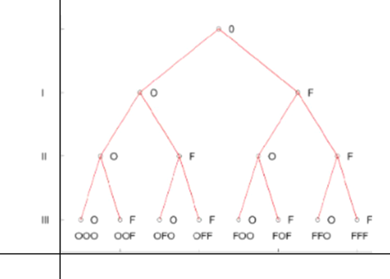
Hence, a tree to represent the possible configurations for these three switches is as follow:

J Susan Milton Introduction To Probability And Statistics Chapter 1 Page 19 Exercise 18 Problem 38
Given – An electrical control panel has three toggle switches labeled I, II, and III each of which can be either on (O) or off(F).
To find – List the elements of the sample space generated by the tree.
From the tree diagram we see that the sample space and sample points are S {OOO,OOF,OFO,OFF,FOO,FOF,FFO,FFF}
Hence, from the elements of the sample space generated by the tree are S = {OOO,OOF,OFO,OFF,FOO,FOF,FFO,FFF}
J Susan Milton Introduction To Probability And Statistics Chapter 1 Page 19 Exercise 19 Problem 39
Given : An electrical control panel has three toggle switches labeled I, II, and III each of which can be either on (O) or off (F).
To find – What is the name given to an event such as D?
Event such as event D = 0 is called aa impossible event.
Hence, from the above explanation Event such as event D = 0 is called a impossible event.
Page 19 Exercise 19 Problem 40
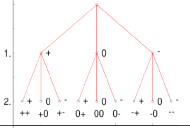
Given: Two items are randomly selected one at a time from an assembly line and classed as to whether they are of superior quality(+), average quality (0), or inferior quality (−)
To find – Construct a tree for this two-stage experiment.
For each of the two items we have tree oscillates. superior quality (+) average quality (0) or inferior quality (-) .
Thus the tree diagram a given with:

Hence, tree for this two-stage experiment is as follow
J Susan Milton Introduction To Probability And Statistics Chapter 1 Page 19 Exercise 19 Problem 41
Given: Two items are randomly selected one at a time from an assembly line and classed as to whether they are of superior quality (+), average quality (0), or inferior quality (-)
To find – List the elements of the sample space generated by the tree.
From the tree diagram, we concluded that to sample space and sample points are S = {++,+0,+−,0+,00,0−,−+,−0,−−}
Hence, the elements of the sample space generated by the tree is as follow S = {++,+0,+−,0+,00,0−,−+,−0,−−}
Page 19 Exercise 19 Problem 42
Given: Two items are randomly selected one at a time from an assembly line and classed as to whether they are of superior quality (+), average quality (0), or inferior quality(−)
To find – List the sample points that constitute the events
A: The first item selected is of inferior quality
B: The quality of each of the items is the same
C: The quality of the first item exceeds that of the second
Using Page 19 Exercise 19 Problem 40 and Page 19 Exercise 19 Problem 41 we have
A = The first item selected is of inferior equal = {−+,−0,−−}
B = The quality of each of the items is the same = {++,00,−}
C = The quality of the First term exceeds that of the second = {+0,+−,0−}
Hence, the sample points that constitute the event are as follow:
A: The first item selected is of inferior quality ={−+,−0,−}
B: The quality of each of the items is the same={++,00,−−}
C: The quality of the first item exceeds that of the second ={+0,+−,0−}
J Susan Milton Introduction To Probability And Statistics Chapter 1 Page 20 Exercise 20 Problem 43
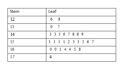
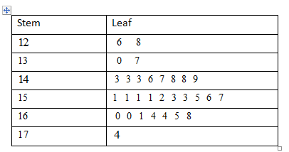
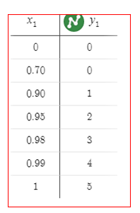
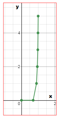
Given: An experiment consists of selecting a digit from among the digits 0 to 9 in such a way that each digit has the same chance of being selected as any other.
We name the digit selected A.
These lines of code are then executed.
IF A < 2 THEN B = 12; ELSE B = 17
IFB = 12 THEN C = A − 1; ELSE C = 0
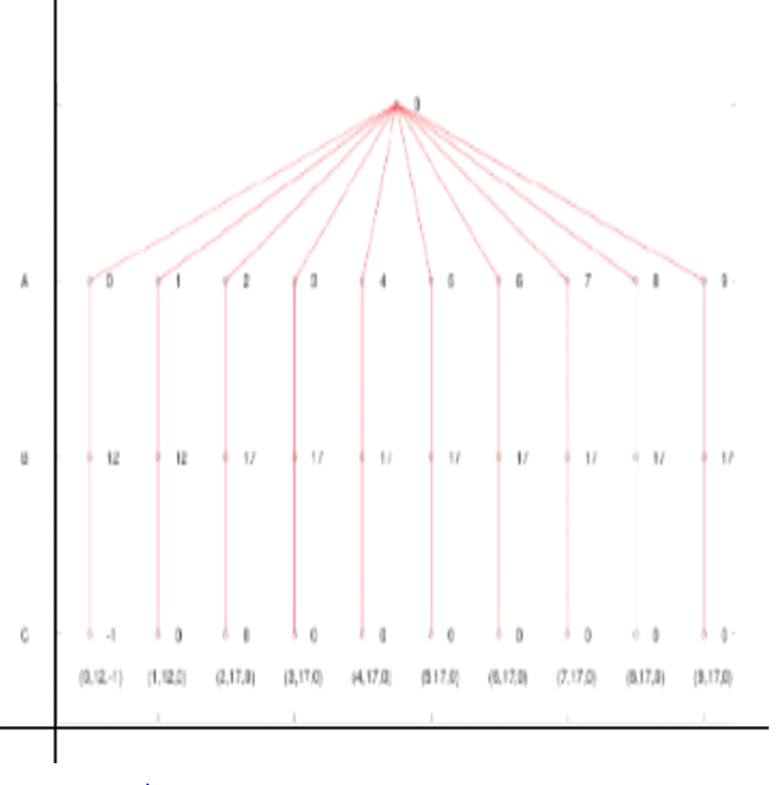
To find – Construct a tree to illustrate the ways in which values can be assigned to the variables A, B, and C
From above given coordinate we have drawn a diagram :
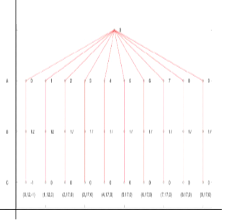
Hence: A tree to illustrate the ways in which values can be assigned to the variables A, B, and C
J Susan Milton Introduction To Probability And Statistics Chapter 1 Page 20 Exercise 20 Problem 44
Given: An experiment consists of selecting a digit from among the digits 0 to 9 in such a way that each digit has the same chance of being selected as any other.
We name the digit selected A.
These lines of code are then executed.
IF A <2 THEN B = 12; ELSE B = 17
IF B = 12 THEN C = A−1; ELSEC = 0
To find – Find the sample space generated by the tree.
From the tree diagraram, we see that the sample space and sample points are
S−{(0,12,−1),(1,12,0),(2,17,0),(3,17,0),(4,17,0),(5,17,0),(6,17,0),(7,17,0),(3,17,0),(9,17,0)\}
Hence, from the above explanation the sample space generated by the tree is as follow S−{(0,12,−1),(1,12,0),(2,17,0),(3,17,0),(4,17,0),(5,17,0),(6,17,0),(7,17,0),(3,17,0),(Officials at Nuclear Regulatory commission estimated the probability of such an accident occurring in the United States before the year to be by using Classical Method.9,17,0)\}
J Susan Milton Introduction To Probability And Statistics Chapter 1 Page 20 Exercise 20 Problem 45
Given: An experiment consists of selecting a digit from among the digits 0 to 9 in such a way that each digit has the same chance of being selected as any other. We name the digit selected A.
These lines of code are then executed.
IF A < 2 THEN B = 12; ELSE B = 17
IF B = 12 THEN C = A-1; ELSE C = 0
To find –Find the probability that A is an even number.
The probability that A is an even number is the probability that A will be 0,2,4,6 or 8. so, there are five possibilities for A to be an even number and five to be an odd number.
Thus the probability that A is are even number is
5.\(\frac{1}{10}\) = \(\frac{1}{2}\)
Hence, from the above explanation the probability that A is an even number is 5.\(\frac{1}{10}\) = \(\frac{1}{2}\)