J. Susan Milton

• Chapter 1 Introduction To Probability And Counting Exercises
• Chapter 2 Some Probability Laws Exercises
• Chapter 3 Discrete Distributions Exercises
• Chapter 4 Continuous Distributions Exercises
• Chapter 5 Joint Distributions Exercises

• Chapter 6 Descriptive Distributions Exercises
• Chapter 7 Estimation Descriptive Distributions Exercises
• Chapter 8 Inferences On The Mean And Variance Of A Distribution Exercise

J.Susan Milton Introduction To Probability And Statistics Principles And Applications Chapter 8 Inferences On The Mean And Variance Of A Distribution

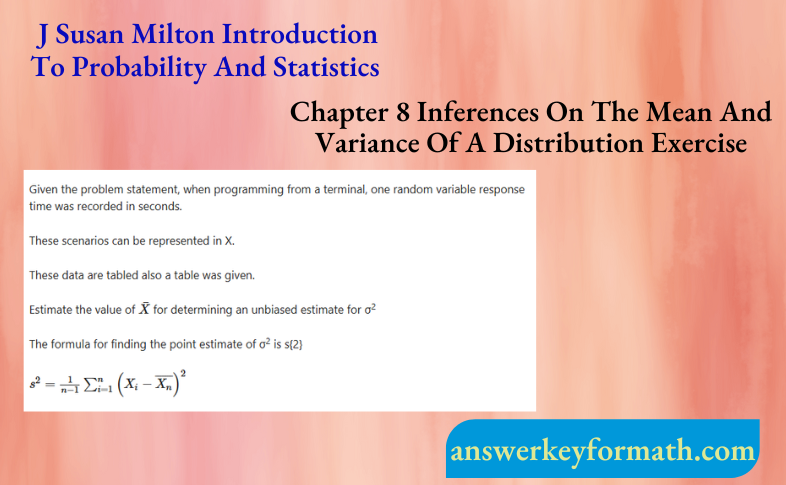
Introduction To Probability And Statistics Chapter 8 Exercises Solutions Page 263  Exercise 1  Problem 1

Given problem statement, when programming from a terminal, one random variable response time was recorded in seconds.

These data are tabled also a table was given.

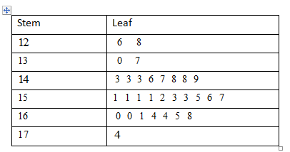
Next draw the stem and leaf diagram and assume the normality is reasonable or not

Stem and leaf plot response time N = 30

Leaf unit = 0.010

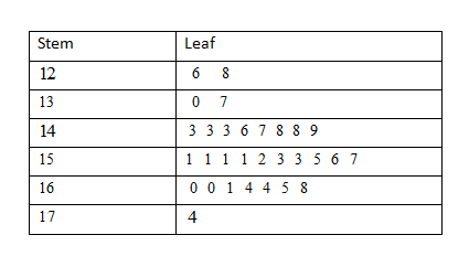
Therefore, the step plot shows the data is equally distributed on both sides. So, the assumptions of normality appear reasonable.

Read and Learn More J Susan Milton Introduction To Probability And Statistics Solutions

J.Susan Milton Introduction To Probability And Statistics Principles And Applications Chapter 8 Page 263  Exercise 1  Problem 2

Given: When programming from a terminal, one random variable response time was recorded in seconds.

These scenarios can be represented in X.

n = 30

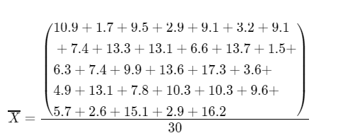
Determine the \(\bar{X}\) value

\(\bar{X}\)n = \(\left(\begin{array}{l}
1.48+1.26+1.52+1.56+1.48+1.46+1.30+1.28+ \\
1.43+1.43+1.55+1.57+1.51+1.53+1.68+1.37+ \\
1.47+1.61+1.49+1.43+1.64+1.51+1.60+1.65+ \\
1.60+1.64+1.51+1.51+1.53+1.74
\end{array} 30\right.\)

Therefore, an unbiased point estimate for σ²  is 0.0129

J.Susan Milton Introduction To Probability And Statistics Principles And Applications Chapter 8 Page 263  Exercise 1  Problem 3

From previous problem the point estimate of σ² is s² was obtained and using this value to find a 95 confidence interval for σ²

First determine the value of α

α = 1 − confidence level

Given :

From previous problem the point estimate of σ² is s² = 0.0129

Find the value of α is

​α = 1 − 95

α =  0.05
​
n =  30

Find a 95 confidence interval for σ²

Formula is , L₁ ≤ σ² L₂

Using chi-square distribution table to find a probability value with corresponds to degrees of freedom.

Probability value0.025 that corresponds to 29 degrees of freedom is 45.7

Probability value 0.0975  that corresponds to 29 degrees of freedom is 16

Determine the confidence interval for σ²

0.00082 ≤ σ²  0.0234

Hence, 95 confidence interval for σ² is (0.0082,0.0234)

Therefore,95 confidence interval for σ2 is (0.0082,0.0234)

J.Susan Milton Introduction To Probability And Statistics Principles And Applications Chapter 8 Page 263  Exercise 1  Problem 4

From previous problem the point estimate for σ²

Was obtained and using this value to find a 95 confidence interval for σ

First determine the value of α

α = 1 − confidence level

Given :

From previous problem the point estimate for σ² is 0.0129

Find the value of α is  α = 1−95

α = 0.05

n = 30

Find a 95 confidence interval for σ formula is

Using chi-square distribution table to find a probability value with corresponds to degrees of freedom.

Probability value0.95 that corresponds to 29 ,degrees of freedom is 45.7

Probability value 0.025 that corresponds to 29 degrees of freedom is 16

Determine the confidence interval for σ

​\(\sqrt{\frac{(30-1)(0.0129)}{45.7}} \leq \sigma \leq \sqrt{\frac{(30-1)(0.0129)}{16.0}}\)

0.091 0.091 ≤ σ ≤0.153

Hence, 95 confidence interval for σ is (0.091,0.153)

Therefore, 95 confidence interval for σ is (0.091,0.153)

J.Susan Milton Introduction To Probability And Statistics Principles And Applications Chapter 8 Page 263  Exercise 2  Problem 5

Given problem statement, highway engineers have found a sign at night and it depends on its surround luminance.

These scenarios can be represented in X.

These surround luminance data are tabled also a table was given.

Estimate the value of X

For determine an unbiased estimate for σ²

Formula for find the point estimate of σ² is s²

s² \(=\frac{\sum\left(X_i-\bar{X}\right)^2}{n-1}\)

Given : Highway engineers have found a sign at night and it depends on its surround luminance.

These scenario can be represented in X.

n = 30

Determine the \(\bar{X}\) value

\(\bar{X}\) = \(\frac{258.6}{30}\)

\(\bar{X}\) = 8.62

The point estimate for σ²  is

s² = \(
\frac{\sum\left(X_i-\bar{X}\right)^2}{n-1}\)

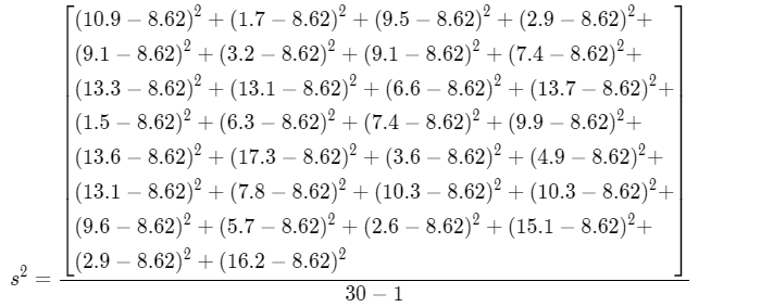
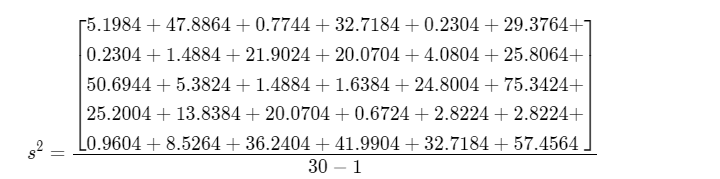
s² = \(\frac{592.428}{29}\)

s² = 20.428

Therefore, an unbiased point estimate for σ²  is, 20.428

J.Susan Milton Introduction To Probability And Statistics Principles And Applications Chapter 8 Page 263  Exercise 2  Problem 6

From the previous problem the point estimate for σ²

was obtained and using this value to find a 90 confidence interval for σ.

First determine the value of α, α = 1− confidence level

Given :

From previous probelm the point estimate for σ² is

20.428

Find the value of α is

​α = 1 − 90

α = 0.10

n = 30

Find a 90 confidence interval for σ²

Formula is

L₁ ≤ σ² ≤ L₂

Using chi-square distribution table to find a probability value with corresponds to degrees of freedom.

Probability value 0.05 that corresponds to 29 degrees of freedom is  42.557

Probability value 0.95 that corresponds to 29 degrees of freedom is  17.7084

Determine the confidence interval for σ²

​\(\frac{(30-1)(20.428)}{42.557} \leq \sigma^2 \leq \frac{(30-1)(20.428)}{17.7084}\)
​

\(\frac{5924.12}{42.557} \leq \sigma^2 \leq \frac{5924.12}{17.7084}\)

13.9204 ≤ σ² ≤ 33.4537

Hence, 90 confidence interval for σ² is (13.9204,33.4537)

Determine the confidence interval for σ

3.731 ≤ σ² ≤ 5.784

Hence, 90 confidence interval for σ is  (3.731,5.784)

Therefore, 90 confidence interval for σ is  (3.731,5.784)

J.Susan Milton Introduction To Probability And Statistics Principles And Applications Chapter 8 Page 264   Exercise 3   Problem 7

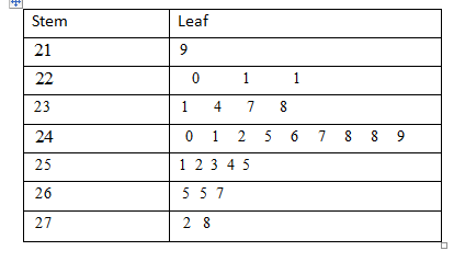
Given problem statement, Two voltage technique is used to analyze the crystals. Using electron microprobe to measure both quantitative and qualitative measurements.

These data are tabled also a table was given.

Next draw the stem and leaf diagram and assume the normality is reasonable or not.

Given :

Stem and leaf plot measurement  N = 27

The values have been multiplied by 100

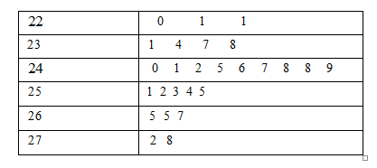
Therefore, the step plot shows the data is equally distributed on both sides. So, the assumptions of normality appear reasonable.

J.Susan Milton Introduction To Probability And Statistics Principles And Applications Chapter 8 Page 264  Exercise 3  Problem 8

Given problem statement, two voltage technique is used to analyze the crystals.

Using electron microprobe to measure both quantitative and qualitative measurements. These scenarios can be represented in X.

These data are tabled also a table was given.

Estimate the value of \(\bar{X}\) for determine an unbiased estimate for σ²

Formula for find the point estimate for σ² is

Given: Two voltage technique is used to analyze the crystals. Using electron microprobe to measure both quantiative and qualiitiative measurements.

These scenario can be represented in X.

n = 27

Determine the \(\bar{X}\) value

\(\bar{X}\) = \(\frac{\sum X_i}{n}\)

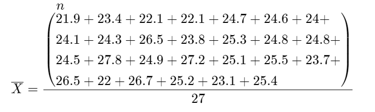
\(\bar{X}\) = \(\frac{663.9}{27}\)

\(\bar{X}\) = 24.59

The point estimate for σ² is

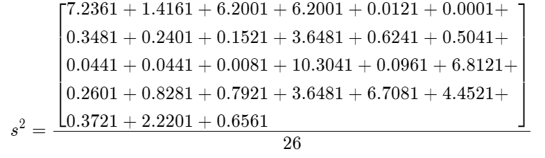
s² = \(\frac{63.8267}{26}\)

s² = 2.455

Therefore, an unbiased point estimate for σ²  is, 2.455

J.Susan Milton Introduction To Probability And Statistics Principles And Applications Chapter 8 Page 264  Exercise 4  Problem 9

Given problem statement, find the one-sided confidence interval for the upper bound.

Also, an interval in the form of [0,L].

Finally prove that the upper bound confidence interval

L = \(\frac{(n-1) s^2}{\chi_{1-\alpha}^2}\)

Given:

Find an interval in the form of  P[σ² ≤ L] = 1 − α

That means Confidence level = 1 − α

Form the diagram, the evidence is

Determine the confidence interval for σ²

P \(\left(\chi_{1-\alpha}^2 \leq \frac{(n-1) s^2}{\sigma^2}\right)\) = 1 − α
​

P \(\left(\sigma^2 \leq \frac{(n-1) s^2}{\chi_{1-\alpha}^2}\right)\) = 1 − α

Hence \(=\frac{(n-1) s^2}{\chi_{1-\alpha}^2}\)

Therefore, the confidence interval for upper bound is \(=\frac{(n-1) s^2}{\chi_{1-\alpha}^2}\) and its proved.

J.Susan Milton Introduction To Probability And Statistics Principles And Applications Chapter 8 Page 265  Exercise 5  Problem 10

Given problem statement, Robotic technology was explained.

The Robots are used to apply adhesive to a specified location.

These location data are tabled also a table was given.

Next draw the stem and leaf diagram and assume the normality is reasonable or not.

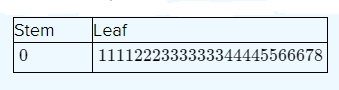
Given :

Stem and leaf plot measurement N = 25

The values have been multiplied by 1000

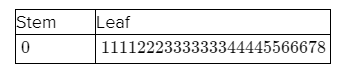
Therefore, the step plot shows the data is equally distributed on both sides. So, the assumptions of normality appear reasonable.

J.Susan Milton Introduction To Probability And Statistics Principles And Applications Chapter 8 Page 265  Exercise 5  Problem 11

Given problem statement, Robotic technology was explained.

The Robots are used to apply adhesive to a specified location. These scenarios can be represented in X.

These location data are tabled also a table was given.

Estimate the value of \(\bar{X}\) For determine an unbiased estimate for σ²

Formula for find the point estimate for σ² is

Given : Robotic technology was explained.

The Robots are used to apply adhesive to a specified location.

These scenarios can be represented in X

n = 27

Determine the \(\bar{X}\) value

\(\bar{X}\) = \(\frac{\sum X_i}{n}\)

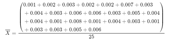
\(\bar{X}\) =\(\frac{0.09}{25}\)

\(\bar{X}\) = 0.0036

The point estimate for  σ² is

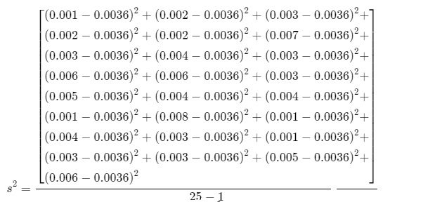
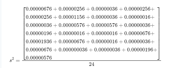
s² = \(\frac{0.00009}{24}\)

s² = 0.00000375

Therefore, an unbiased point estimate for σ² is, 0.00000375

J.Susan Milton Introduction To Probability And Statistics Principles And Applications Chapter 8 Page 265  Exercise 6  Problem 12

Initially understand the theorems and using the theorem to prove that mean and variance values such as E[S² ]= σ² and Var S²

= \(\frac{2 \sigma^4}{(n-1)}\)

Show that X be a random variable. The mean and variance is
​​E[S² ]= σ²

Var S² = \(\frac{2 \sigma^4}{(n-1)}\)

From S² is an unbiased estimator for σ². Hence? E[S²] = σ²

From using of formula \(\frac{(n-1) S^2}{\sigma^2} \sim \chi_{(n-1)}\)

​The variance of the chi squared distribution is n 2(n−1)

Now

Var [ \(\frac{(n-1) S^2}{\sigma^2}\)] = 2(n – 1)

\(\frac{(n-1)^2}{\sigma^4}\)Var S² = 2(n – 1)

Var S² = 2(n – 1)\(\frac{\sigma^4}{(n-1)^2}\)

Var s² =\(\frac{2 \sigma^4}{(n-1)}\)

Therefore, X be a random variable then the mean and variance E[S² ]= σ²,Var S² \(\frac{2 \sigma^4}{(n-1)}\) and its proved.

J.Susan Milton Introduction To Probability And Statistics Principles And Applications Chapter 8 Page 265  Exercise 7  Problem 13

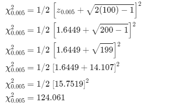
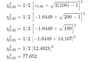
Given Samples: χ_0.005 and χ_0.95

Formula for find chi squared points: \(\chi_r{ }^2=1 / 2\left[z_r+\sqrt{2 \gamma-1}\right]^2\)

Using above formula to determine the approximate points of the given samples.

Given : χ_0.005 and χ_0.95

Formula for approximate the chi squared points \(\chi_r{ }^2=1 / 2\left[z_r+\sqrt{2 \gamma-1}\right]^2\)

r is significance level and γ is the degrees of freedom

Approximate the points for  χ_0.005

Approximate the points for χ_0.95

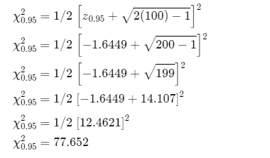
Therefore, approximated points of  χ_0.005  and  χ_0.95  is 124.061  and 77.652

J.Susan Milton Introduction To Probability And Statistics Principles And Applications Chapter 8 Page 265  Exercise 7  Problem 14

Given: Standard deviation value is s = 7.5 and sample size is n = 150

Using above values to find the confidence interval on deviation.

Formula for find the confidence interval for deviation

Given:   Standard deviation and sample sizes are included below

s = 7.5

n = 150

Formula for find interval

Determine the interval for χ_0.025

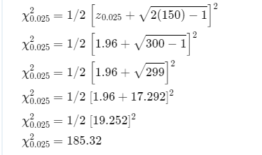
Determine the interval for χ_0.025

Confidence interval is

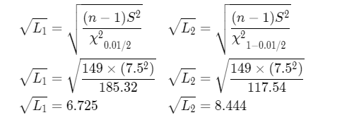
Hence, 95 % confidence interval on the standard deviation is (6.725,8.444)

Therefore,95 % the confidence interval on the standard deviation is(6.725,8.444)

J.Susan Milton Introduction To Probability And Statistics Principles And Applications Chapter 8 Page 266  Exercise 8  Problem 15

Given: Standard deviation value is s = 0.01 and sample size is n = 100

Using above values to find the confidence interval for deviation One sided confidence interval

Given : Standard deviation and sample size is

​s = 0.01

n = 100

Formula for find interval

Chi squared points can be approximated by the formula

Approximate the points for χ_0.95

Determine the confidence interval

= 0.0113

Hence, 95 % confidence interval on the standard deviation is (0,0.0113)

Therefore, 95 % confidence interval on the standard deviation is (0,0.0113)

J.Susan Milton Introduction To Probability And Statistics Principles And Applications Chapter 8 Page 266  Exercise 9  Problem 16

Given: t.05 (γ = 8)

In T  Distribution table, the cumulative probability values are given.

If find a critical value, look up the confidence interval in the bottom row of the table.

From T distribution table the row locates 8 and the column of P[Tr ≤ t]  locate 0.95 which corresponds to the critical value is 1.8595

Hence, the value of t.05 (γ = 8) is 1.8595

Therefore, the value of  t.05(γ = 8) is 1.8595

J. Susan Milton Chapter 8 Inferences On Mean And Variance Answers Page 266  Exercise 9  Problem 17

Given: t.95 (γ = 8)

In T Distribution table, the cumulative probability values are given.

If find a critical value, look up the confidence interval in the bottom row of the table.

From T distribution table the row locates 8 and the column of P[Tr ≤ t] locate 0.95 which corresponds to the critical value is −1.8595

Therefore, the value of t.95 (γ = 8)  is−1.8595

J.Susan Milton Introduction To Probability And Statistics Principles And Applications Chapter 8 Page 266  Exercise 9  Problem 18

Given:  t 0.975 (γ = 12)

In T Distribution table, the cumulative probability values are given.

If find a critical value, look up the confidence interval in the bottom row of the table.

From T distribution table the row locates 12 and the column of P[Tr  ≤ t] locate 0.975 which corresponds to the critical value is −2.1788

Hence, the value of  t.975 (γ = 12) is −2.1788

Therefore, the value of t 975 (γ = 12) is −2.1788

Solutions To Inferences On Mean And Variance Exercises Chapter 8 Susan Milton Page 265  Exercise 10  Problem 19

In this given question, t value is .05.

In this given question, γ value is 50

Have to find a probability for given t value with given γ value.

Point degree of freedom and search for a given t value.

Given t value = .05.

γ = 50.

By using the t table, t⋅05 (γ = 50) = 1.6759

Hence, the probability of given t value ⋅05 with degree of freedom γ = 50 is 1.6759.

J.Susan Milton Introduction To Probability And Statistics Principles And Applications Chapter 8 Page 265  Exercise 10  Problem 20

In this given question, t value is .025.

In this given question, y value is 75.

Have to find a probability for given t value with given γ value.

Point degree of freedom and search for a given t value.

Given t

value  t  = .025

γ = 75

By using the t table, t  = .025

(γ = 75) = 1.9921

Hence, the probability of given t value .025 with degree of freedom γ = 75 is 1.9921

Chapter 8 Inferences on Mean and Variance examples and answers Susan Milton Page 265  Exercise 10  Problem 21

In this given question, t value is 0.1.

In this given question, γ value is 200.

Have to find a probability for given t value with given γ value.

Point degree of freedom and search for a given t value.

Given

t value = 0.1

γ = 200

By using the t table

t 0⋅1 (γ = 200) = 1.2858

Hence, the probability of given t value 0.1 with degree of freedom γ = 200 is 1.2858

J.Susan Milton Introduction To Probability And Statistics Principles And Applications Chapter 8 Page 266 Exercise 11 Problem 22

In this question, the given data is \(\sum_{i=1}^{20} x_i\) = 25.792 and

\(\sum_{i=1}^{20} x_i^2\) = 33. 261596

Have to find \(\bar{X}\) , s² , s

\(\bar{X}\) = \(\frac{\sum x_i}{n}\)

s2 = \(\frac{1}{n-1}\left(\sum x_i^2-n(\bar{X})^2\right)\)

s = \(\sqrt{s^2}\)

Given

\(\sum_1^{15} x_i\)  =  0.07

\(\sum_1^{15} x_i^2\) = 0.0489

n = 15

\(\bar{X}\) = \(\frac{\sum x_i}{n}\)

\(\bar{X}\)  = \(\frac{0.07}{15}\)

\(\bar{X}\)  = 0.00467

= \(\frac{1}{15-1}\left(0 \cdot 0489-15(0 \cdot 00467)^2\right)\)

=  \(\frac{1}{14}(0 \cdot 0489-0 \cdot 000327)\)

= \(\frac{0.048573}{14}\)

=   0.0034695

s = \(\sqrt{s^2}\) = \(\sqrt{0.0034695}\)

s  =  0.0589

Hence, the Value of \(\bar{X}\),s ², s are 0⋅00467, 0⋅0034695,0⋅0589 respectively.

J.Susan Milton Introduction To Probability And Statistics Principles And Applications Chapter 8 Page 266  Exercise 11  Problem 23

To find 95 % confidence interval 100(1 − α)

\(\bar{X} \pm t_{\frac{\alpha}{2}, \frac{n-1 s}{\sqrt{n}}}\) = 0.00467 \(\pm t_{0.05, \frac{15-10.0589}{\sqrt{5}}}\)

​=  0⋅00467 ± 1.7693 × 0.0152

=  0.00467 ± 0.0269

=  (0⋅00467 − 0.0269, 0.00467 + 0.0269)

=  (−0.02223, 0.03157)
​
Hence,95 % confidence interval on the mean outside diameter of the pipes is(−0.02223,0.03157)

J.Susan Milton Introduction To Probability And Statistics Principles And Applications Chapter 8 Page 266  Exercise  11  Problem 24

The makers of this pipe claim that the mean outside diameter is 1.29, so an average overestimate is 0.05.

The average overestimates the distance by 0.05 which is not reasonable.

Because the overestimates do not lie within 90 confidence interval.

Hence, the confident interval does not lead to suspect this responded.

J.Susan Milton Introduction To Probability And Statistics Principles And Applications Chapter 5 Joint Distributions 

Introduction To Probability And Statistics Chapter 5 Exercises Solutions Page 169  Exercise 1  Problem 1

In Given problem, is a hypergeometric distribution.

Hypergeometric distribution: A random variable X has a hypergeometric distribution with parameters N,n and r if its density is given by

f(x) = \(\frac{\left(\begin{array}{l}
r \\
x
\end{array}\right)\left(\begin{array}{l}
N-r \\
n-x
\end{array}\right)}{\left(\begin{array}{l}
N \\
n
\end{array}\right)}\)

Max [0,n−(N−r)] ≤ x ≤ min(n,r)

Given table

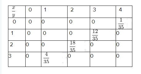
Find the probability for hypergeometric function

Using given statement to get a required probability such as, N = 7,r = 3

P(X = x) = \(\frac{\left(\begin{array}{l}
r \\
x
\end{array}\right)\left(\begin{array}{l}
N-r \\
n-x
\end{array}\right)}{\left(\begin{array}{l}
N \\
n
\end{array}\right)}\)

Putx = 0 in above equation

P(X = x) = \(\frac{\left(\begin{array}{l}
3 \\
0
\end{array}\right)\left(\begin{array}{l}
7-3 \\
4-0
\end{array}\right)}{\left(\begin{array}{l}
7 \\
4
\end{array}\right)}\)

P(X = x) = \(\frac{1}{35}\)

Therefore, the probability for a hypergeometric function value is \(\frac{1}{35}\) and the table values are verified.

Read and Learn More J Susan Milton Introduction To Probability And Statistics Solutions

J.Susan Milton Introduction To Probability And Statistics Principles And Applications Chapter 5 Page 169  Exercise 1  Problem 2

Hence, the marginal density was obtained and the variable Y is the Continuous Random Variable.

Therefore, the marginal density was obtained and the variable Y is the Continuous Random Variable.

J. Susan Milton Joint Distributions Chapter 5 Answers Page 169  Exercise 1 Problem 3

If two random variables are independent then it satisfies the following conditions,

​1. P(x/y) = P(x)

2. P(x ∩ y) = P(x) ∗ P(y)
​
Also, the joint distribution of a function is f_xy (x,y) = f_x (x) f_y(y)

Two random variables are independent, if the value of one variable does not change the probability value of another variable.

Therefore, If two random variables for independent then satisfies a condition 1. P(x∣y) = P(x) , 2. P(x∩y) = P(x)∗ P(y)

​

J.Susan Milton Introduction To Probability And Statistics Principles And Applications Chapter 5 Page 169   Exercise 2   Problem 4

Given problem, f_xy(x,y) = 1/n²

If determine a function has to be joint density function satisfies the below condition,\(\sum_x \sum_y f_{X Y}(x, y)\) = 1

The values of X and Y between

​x = 1,2,3 ,…., n

y = 1,2,3, …., n

​Given: f_xy(x,y) = 1/n²

Find joint density function

\(\sum_x \sum_y f_{X Y}(x, y)\) = 1

Hence, a given function is discrete joint density function and the condition is satisfied.

Therefore, the function is a discrete joint density function and the condition x \(\sum_x \sum_y f_{X Y}(x, y)\) = 1 is satisfied.

Solutions To Joint Distributions Exercises Chapter 5 Susan Milton Page 169  Exercise 2  Problem 5

Given problem, fxy(x,y) = 1/n²

If determine a function has to be joint density function satisfies the below condition,\(\sum_x \sum_y f_{X Y}(x, y)\)= 1

The values of X and Y between

​x = 1,2,3, …., n

y = 1,2,3, …., n

Given: fxy(x,y)=1/n²

Find joint density function

Using given function to get a marginal density

Find the marginal density of X

Determine the marginal density of Y

\(f_Y(y)=\frac{1}{n^2} \sum_1^n 1\)

 \(f_Y(y)=\frac{1}{n^2}(n)\)

 \(f_Y(y)=\frac{1}{n}\)

Therefore, the marginal densities of a given function both X and Y is  \(\frac{1}{n}\)

J.Susan Milton Introduction To Probability And Statistics Principles And Applications Chapter 5 Page 169  Exercise 2  Problem 6

If two random variables are independent then it satisfies the following conditions,

​1. P(x∣y) = P(x)

2. P(x ∩ y) = P(x) ∗ P(y)
​
Also, the joint distribution of a function is

fxy(x,y) = f_x(x) f_y(y)

Two random variables are independent, if the value of one variable does not change the probability value of another variable.

Given problem,{{f}{XY}}(x,y) = 1/n²

The marginal densities of a given function both X
and Y is \(f_Y(y)=\frac{1}{n}\).

Hence, the values are independent.

Therefore, the given function marginal densities of both X and Y is \(f_Y(y)=\frac{1}{n}\) and independent.

Chapter 5 Joint Distributions Examples And Answers Susan Milton Page 169  Exercise 3  Problem 7

Given problem ,f_xy(x,y) = 2/n(n+1)

If determine a function has to be joint density function satisfies the below condition \(f_Y(y)=\frac{1}{n}\).

The values of X and Y between

​x = 1,2,3,….,n

y = 1,2,3,….,n
​
Given: f_xy (x,y) = 2/n(n + 1)

Find joint density function

Sum of first n integers is given by \(\frac{n(n+1)}{2}\)

\(\sum_{y=1}^n \sum_{x=1}^n f_{X Y}(x, y)\) =  1

Hence, a given function is discrete joint density function and the condition is satisfied.

Therefore, the function is a discrete joint density function and the condition \(\sum_{y=1}^n \sum_{x=1}^n f_{X Y}(x, y)\)= 1 is satisfied.

J.Susan Milton Introduction To Probability And Statistics Principles And Applications Chapter 5 Page 169  Exercise 3  Problem 8

Given problem, f_xy (x,y) = 2/n(n + 1)

If determine a function has to be joint density function satisfies the below condition \(f_Y(y)=\frac{1}{n}\).

The values of X and Y between

​x = 1,2,3,….,n

y = 1,2,3,….,n

Using given function to get a marginal density

Find the marginal density of X,

Determine the marginal density of Y

Therefore, the marginal densities of a given function both X and Y \(f_X(x)=\frac{2}{(n+1)}\)

J.Susan Milton Introduction To Probability And Statistics Principles And Applications Chapter 5 Page 169  Exercise 3  Problem 9

If two random variables are independent then it satisfies the following conditions,

​1. P(x∣y) = P(x)

2. P(x∩y) = P(x) ∗ P(y)
​
Also, the joint distribution of a function is

f_xy(x,y) = f_x(x) f_y(y)

Two random variables are independent, if the value of one variable does not change the probability value of another variable.

Given problem, f_xy (x,y) = 2/n(n + 1)

The marginal densities of a given function both X and Y is \(f_X(x)=\frac{2}{(n+1)}\)

Hence, the values are independent.

Therefore, the given function marginal densities of both X and Y is \(f_X(x)=\frac{2}{(n+1)}\) and its independent.

Probability And Statistics J. Susan Milton Chapter 5 Solved Step-By-Step Page 170  Exercise 4  Problem 10

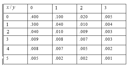
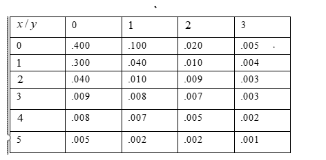
In Given table,X represents the number of syntax errors and Y represents the number of errors in logic.

Problem statement: Determine the probability for selected program have neither of these errors.

Given table

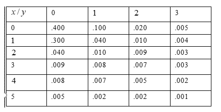
In above table,X represents the number of syntax errors and Y represents the number of errors in logic.

Find the probability

Using given statement to get a required probability such as, p(x = 0,y = 0)

Hence, the value of p(x = 0,y = 0) is 0.4

Hence, the probability that selected program have neither these types of errors as 0.4

Therefore, the probability that selected program have neither these types of errors as 0.4

J.Susan Milton Introduction To Probability And Statistics Principles And Applications Chapter 5 Page 170  Exercise 4  Problem 11

In Given table,X represents the number of syntax errors and Y represents the number of errors in logic.

Problem statement: Determine the probability for selected program at least one syntax error and at most one error in logic.

Given table,In above table,X represents the number of syntax errors and Y

Find the probability

Using given statement to get a required probability such as,

P[X ≥ 1 and Y ≤ 1]

P[X ≥ 1and Y ≤ 1]

[P(X = 1,Y = 0) +  P(X = 2,Y = 0) + P(X = 3,Y = 0)

+ P(X = 4,Y = 0) + P(X = 5,Y = 0) + P(X = 1,Y = 1)

+ P(X = 1,Y = 2) +  P(X = 1,Y = 3) + P(X = 1,Y = 4)

+ P(X = 1,Y = 5)]

P[X ≥ 1and Y ≤ 1]​ = 0.300 + 0.040 + 0.009 + 0.008 + 0.005 + 0.040 + 0.010+ 0.008 + 0.007 + 0.002

P[X ≥ 1and Y ≤ 1] = 0.429

Hence, the probability for selected at least one syntax error and at most one error in logic is 0.429

Therefore, the probability for selected at least one syntax error and at most one error in logic is 0.429

J.Susan Milton Introduction To Probability And Statistics Principles And Applications Chapter 5 Page 170  Exercise 4  Problem 12

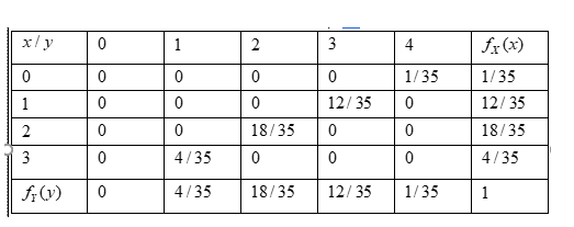
Using given table values for determine the marginal density of the function.

If two random variables with joint density fXY then the marginal density for X denoted as f_x given by

The mariginal density for y denoted as

Given table

In above table, X represents the number of syntax errors and y represents the number of errors in logic.

Using Given table, sum all values for determine a marginal density

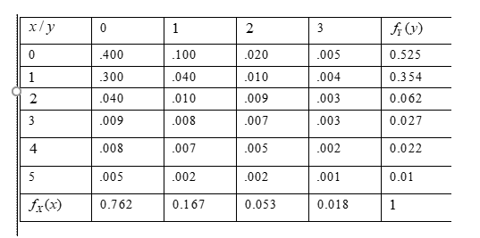
Hence, the marginal density was obtained

Therefore, the marginal density for both values are obtained in above table.

J.Susan Milton Introduction To Probability And Statistics Principles And Applications Chapter 5 Page 170  Exercise 5  Problem 13

On previous example to get a function is, f_xy(x,y)= \(\frac{1.72}{x}\)

If determine a function has to be joint density function satisfies the below condition

The values of $X$ and $Y$ between 27 ≤ y ≤ x ≤ 33

Given: \(f_{X Y}(x, y)=\frac{1.72}{x}\)

Use continuous joint density function to find the value of P[X ≤ 30 and Y ≤ 28]

P[X ≤ 30 and Y≤ 28]= \(\int_{27}^{30} \int_{27}^{28} f_{X Y}(x, y) d x d y\)

Integrate depends on y and apply the limit values in given function

\( = 1.72 \int_{27}^{30} \frac{1}{x}[y]_{27}^{28} d x\)

Integrate depends on x and apply the limit values in given function

P[X ≤ 30 and Y≤28] = 1.72× \([\ln x]_{27}^{30}\)

P[X ≤ 30 and Y≤28]  ​= 1.72(3.4012 − 3.2958)

P[X ≤ 30 and Y≤28]  =  0.1813
​
Therefore, using previous example to find a function as f_xy (x,y)= \(\frac{1.72x}{x}\) and the value of P[X ≤ 30 and Y ≤ 28] is 0.1813.

J.Susan Milton Introduction To Probability And Statistics Principles And Applications Chapter 5 Page 170  Exercise 6  Problem 14

On previous example to get a function is,f _xy(x,y) = \(\frac{c}{x}\)

If determine a function has to be joint density function satisfies the below condition \(\int_{-\infty}^{\infty} \int_{-\infty}^{\infty} f_{X Y}(x, y) d x d y\) = 1

The values of X and Y between 27 ≤ y ≤ x ≤ 33

Given: f_xy (x,y) = \(\frac{c}{x}\)

Use continuous joint density function to find the value of c

\(\int_{-\infty}^{\infty} \int_{-\infty}^{\infty} f_{X Y}(x, y) d y d x\) = 1

​\(\int_{27}^{33} \int_{27}^x \frac{c}{x} d y d x\)= 1

Integrate depends on y and apply the limit values in given function

\(\int_{27}^{33}\left(\frac{c}{x} y\right)_{27}^x d x\) = 1

\(\int_{27}^{33}\left(c-\frac{c}{x}(27)\right) d x\) = 1

Integrate depends on x and apply the limit values in given function

\(\int_{27}^{33} c d x-27 \int_{27}^{33} \frac{c}{x} d x\)= 1

6c − 27c (ln(33)−3ln(3)) = 1

6c − 5.4181c = 1

c = \(\frac{1}{0.5819}\)

c  = 1.72
​
Therefore, using previous example to find a function as f XY(x,y) = \(\frac{1.72}{x}\)with 27 ≤ y ≤ x ≤ 33 and the value of c is 1.72

Online Help For J. Susan Milton Joint Distributions Chapter 5 Exercises Page 170  Exercise 6  Problem 15

On previous example to get a function is \(f_{X Y}(x, y)=\frac{1.72}{x}\)

If determine a function has to be joint density function satisfies the below condition, \(f_X(x)=\int_{-\infty}^{\infty} f_{X Y}(x, y) d y\) 27 ≤ y ≤ x ≤ 33

Given: \(f_{X Y}(x, y)=\frac{1.72}{x}\)

Using given function to get a marginal density

Find the marginal density of X

Integrate depends on Y and apply the limit values in given function

\(f_X(x)=1.72\left(\frac{1}{x}\right)[y]_{27}^{28}\)

Therefore, Therefore, the marginal density for X and the value of P[X≤28] is \(f_{X Y}(x, y)=\frac{1.72}{x}\)

J.Susan Milton Introduction To Probability And Statistics Principles And Applications Chapter 5 Page 170  Exercise 7  Problem 16

Given problem, f_xy (x,y) = c(4x + 2y + 1)

If determine a function has to be joint density function satisfies the below condition

\(\int_{-\infty}^{\infty} \int_{-\infty}^{\infty} f_{X Y}(x, y) d x d y\) = 1

The values of X and Y between

​0 ≤ x ≤ 40

0 ≤ y ≤ 2
​
Given: f_xy (x,y) = c(4x + 2y + 1)

Use continuous joint density function to find the value of c

\(\int_{-\infty}^{\infty} \int_{-\infty}^{\infty} f_{X Y}(x, y) d x d y\) = 1

\(\int_0^{40} \int_0^2 c(4 x+2 y+1) d x d y\) = 1

Integrate depends on y and apply the limit values in given function

\(c \int_0^{40}\left(4 x y+2 \frac{y^2}{2}+y\right)_0^2 d x\) = 1

\(c \int_0^{40}\left(4 x(2)+(2)^2+2\right) d x=\) 1

Integrate depends on x and apply the limit values in given function,

\(c \int_0^{40}(8 x+6) d x\)= 1

\(c\left(\frac{8 x^2}{2}+6 x\right)_0^{40}\)= 1

\(c\left(\frac{8(40)^2}{2}+6(40)\right)\)= 1

6640c  = 1

c = \(\frac{1}{6640}\)

Therefore, the given function fXY (x,y)=c(4x+2y+1) and the value of c is \(\frac{1}{6640}\)= 1

Step-By-Step Guide To Joint Distributions Exercises Chapter 5 Milton Page 170  Exercise 7  Problem 17

To solve this, we need to integrate the PDF where X and Y defined as follow.

​P(x > 20,y ≥ 1)

20 < x ≤ 0,1 ≤ y ≤ 2

P(x > 20,y ≥ 1) = 1 \(\int_1^2 \int_{20}^{40} \frac{1}{6640}(4 x+2 y+1) d x d y\)

P(x > 20,y ≥ 1)  =  \(\frac{1}{6640} \int_1^2\left(\frac{4 x^2}{2}+2 y x+x\right) \int_{20}^{40} d y\)

P(x > 20,y ≥ 1)  = \(\frac{1}{6640} \int_1^2(40 y+2420) d y\)

P(x > 20,y ≥ 1)  = \(\frac{1}{6640} \int_1^2(40 y+2420) d y\)

P(x > 20,y ≥ 1)  = \(=\frac{1}{6640}(2480)\)

P(x > 20,y ≥ 1)  = \(\frac{38}{83}\)

The probability of temperature is P(x > 20,y ≥ 1) =\(\frac{38}{83}\)

J.Susan Milton Introduction To Probability And Statistics Principles And Applications Chapter 5 Page 171  Exercise 8  Problem 18

Note that the integral of a valid joint density is equal to 1.

To verify joint density for a two-dimensional random variable.

f _xy (x,y) =  \([\frac{1}{x}\),o < y < x < 1

That the integral of a valid joint density is equal to 1.

1= \(1\iint_R f_{X, Y}(x, y), o<y<x<1\)

= \(\int_0^1 \int_0^x \frac{1}{x} d y d x\)

= \(\left.\int_0^1\left(\frac{y}{x}\right)\right|_0 ^x d x\)

= \(\left.(x)\right|_0 ^1\)

1 = 1

It is a joint density variable.

Exercise Solutions For Chapter 5 Susan Milton Joint Distributions Page 171   Exercise 8  Problem 19

We can get the probability by integrating it into the following regions.

To find P(X ≤ 0.5 and Y ≤ 0.25)

We can get the probability by integrating it on the following regions

0 < y ≤ 0.25

0.25≤ x < 0.5

Thus, we get that

P(X ≤ 0.5 and Y ≤ 0.25) = \(\int_{0.25}^{0.5} \int_0^{0.25} \frac{1}{x} d y d x\)

P(X ≤ 0.5 and Y ≤ 0.25)  = \(\left.\int_{0.25}^{0.5}\left(\frac{y}{x}\right)\right|_0 ^{0.25} d x\)

P(X ≤ 0.5 and Y ≤ 0.25)  = \(\left.0.25[\ln (x)]\right|_0 ^{0.25}\)

P(X ≤ 0.5 and Y ≤ 0.25)  = 0.25 [(ln(0.5)] − [ln(0.25)]

P(X ≤ 0.5 and Y ≤ 0.25)  = 0.1733

Hence, we have found the answer for P(X ≤ 0.5and Y ≤ 0.25) = 0.1733

J.Susan Milton Introduction To Probability And Statistics Principles And Applications Chapter 5 Page 171  Exercise 9  Problem 20

The marginal density distribution of a subset of a collection of random variables is the probability distribution.

To find the marginal densities for X and Y.

To calculate the marginal density for X, by definition, we have to calculate the integral

By plugging in the values where y is defined and the expression for joint density function, we obtain.

\(f_X(x)=\int_0^2 \frac{x^3 y^3}{16} d y=\frac{x^3}{64}(16-0)=\frac{x^3}{4}\), 0 ≤ x ≤ 2
​

To calculate the marginal density for Y, by definition, we have to calculate the integral

\(\left.f_Y(y)=\int \mathbb{r} f_{(} X, Y\right)(x, y) d x\)
​

By plugging in the values where y is defined and the expression for joint density function, we obtain.

\(f_X(x)=\int_0^2 \frac{x^3 y^3}{16} d y\)
​
\(=\frac{x^3}{64}(16-0)\)

\(=\frac{x^3}{4}\), 0 ≤ x ≤ 2

\(\frac{x^3}{4}\) 0 ≤ x ≤ 2

\(\frac{x^3}{4}\) 0 ≤ x ≤ 2

⇒ \(f_Y(y)=\frac{y^3}{4}, 0 \leq y \leq 2\)

J.Susan Milton Introduction To Probability And Statistics Principles And Applications Chapter 5 Page 171  Exercise 9  Problem 21

The marginal density distribution of a subset of a collection of a random variables is the probability distribution.

To explain if X and Y are independent?

To check if X and Y are independent, we can simply check whether or not the following equation is fulfilled.

f_x,y(x,y) =  f_x(x) f_y(y)

By substituting the calculated expression , we obtain

Hence X and Y are indeed independent.

Hence X and Y are indeed independent.

Page 171  Exercise 9  Problem 22

The marginal density distribution of a subset of a collection of random variables is the probability distribution.

To find P(X ≤ 1)

To find the probability P(X≤1), by definition, we have to calculate integral

P(X≤1) \(=\int_{-\infty}^1 f_X(x) d x\)

By substituting the given expression for the marginal density function and the values where x is defined, we proceed to calculate

P(X ≤ 1) \(\left.=\int_0^{\frac{x 3}{4}} d x=\frac{1}{16}-(1-0)=\frac{(}{1}\right)(16)\)

Therefore, the joint density for (X,Y) is given by \(\frac{1}{6}\)

J.Susan Milton Introduction To Probability And Statistics Principles And Applications Chapter 5 Page 171  Exercise 10  Problem 23

f_x,y(x,y) = c,   20 < x < y < 40 The integral of the PDF should always be equal to l, where x and y is defined.

Thus we get

\(=\int_{20}^{40} \int_{20}^y c d x d y\)
​
\(=c \int_{20}^{40}(y-20) d y\)

= c (200)

= c\(\frac{1}{200}\)

The value of c is c\(\frac{1}{200}\)

Page 171  Exercise 10  Problem 24

The integral of the PDF should always be equal to l, where x and y are defined, then integrating the PDF.

To find the probability that the carrier will pay at least $25 per barrel and the refinery will pay at most $30 per barrel for the oil.

We can express the problem

P(X ≥ 25 and Y ≥ 30)

By integrating the PDF, we get that
​
​P(X ≥ 25 and Y ≥ 30)

​​P(X ≥ 25 and Y ≥ 30\(=\int_{30}^{40} \int_{25}^y \frac{1}{200} d x d y\)

​P(X ≥ 25 and Y ≥ 30) = \(\frac{1}{200} \int_{30}^{40}(y-25) d y\)

​P(X ≥ 25 and Y ≥ 30)= \(\left.\frac{1}{200}\left(\frac{y^2}{2}-25 y\right)\right|_{30} ^{40}\)

​P(X ≥ 25 and Y ≥ 30)= \(\left.\frac{1}{200}\left(\frac{y^2}{2}-25 y\right)\right|_{30} ^{40}\)

​P(X ≥ 25 and Y ≥ 30)= \(\frac{1}{200}\)

​P(X ≥ 25 and Y ≥ 30)= \(\frac{1}{2}\)

P(X ≥ 25 and Y ≥ 30) = \(\frac{1}{2}\)

J.Susan Milton Introduction To Probability And Statistics Principles And Applications Chapter 5 Page 171  Exercise 10  Problem 25

The integral of the PDF should always be equal to l, where x and y are defined, then integrating the PDF.

To find the probability that the price paid by the refinery exceeds that of the carrier by at least $10 per barrel.

We can express the problem

P(Y > X + 10)

Now if we graph the domain, we get

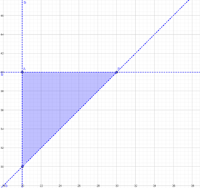
Where

Point A = (20,40)

Point B = (30,40)

Point C = (20,30)

CB  = y − 10

By integrating the PDF
​
​P(Y>X+10)= \(\int_{30}^{40} \int_{25}^y \frac{1}{200} d x d y\)

= \(\frac{50}{200}\)

= 0.25

The probablity is P(Y > X + 10) = 0.25

J.Susan Milton Introduction To Probability And Statistics Principles And Applications Chapter 5 Page 172  Exercise 11 Problem 26

From Continuous Joint density we get that the three properties and identify a function as a density (X₁,X₂,X₃,….. .X_n) f X₁, X₂, X₃ ,. ….. X_n(x₁,x₂,x₃, ….. .x₁ )≥0]−∞<X_i< ∞

For all Xi where i is from 1 to n

\(\int_{-\infty}^{\infty} \int_{-\infty}^{\infty} \int_{-\infty}^{\infty} \cdots \cdots \int_{-\infty}^{\infty}\) f X₁, X₂, X₃ ,…… X₁ (x₁ ,x₂,x₃,……x₁ ) dx₁ dx₂ dx₃……..

P[a ≤ X₁ ≤ b,c ≤ X ≤ d,e ≤ X₃ ≤ f,…..,g ≤ X₁ ≤ h

\(\int_a^b \int_c^d \int_e^f \cdots \cdots \int_g^h\)  f X₁, X₂, X₃ ,…… X(x₁,x₂,x₃,……x_n) dx₁dx₂ dx₃ ………..;. Where a, b, c, …., h are real

Hence, a, b, c, …., h is called the joint density for (X₁ ,X₂,X₃,…..,X_n)

J.Susan Milton Introduction To Probability And Statistics Principles And Applications Chapter 7 Estimation Descriptive Distributions

Introduction To Probability And Statistics Chapter 7 Exercises Solutions Page 221  Exercise 1  Problem 1

Given problem, X₁,X₂,X₃ ,…..,X₂₀

In the given information, the population mean μ and variance σ were given.

Using the given values to find the sample mean and variance value.

Given: The population mean(μ)is 8 and the variance (σ)is 5.

Determine the mean of \((\bar{X})\)

The sample mean \((\bar{X})\) is an unbiased estimator of the population mean(μ)

The mean \((\bar{X})\) of the sample m X₁,X₂,X₃ ,…..,X₂₀   is the population mean.

Hence, the sample mean value is \((\bar{X})\) = 8

Determine the variance of \((\bar{X})\)

var \((\bar{X})\) = \(\frac{\sigma^2}{n}\)

Substitute n = 20 and σ² = 5 in previous term

Var \((\bar{X})\) = \(\frac{5}{20}\)= 0.25

Therefore, the mean and variance of \((\bar{X})\) is Mean: 8 Variance: 0.25

Read and Learn More J Susan Milton Introduction To Probability And Statistics Solutions

J.Susan Milton Introduction To Probability And Statistics Principles And Applications Chapter 7 Page 221  Exercise 2  Problem 2

​
Therefore, an unbiased estimator for the given parameter λs is X. X is the unbiased estimator of λs

J.Susan Milton Introduction To Probability And Statistics Principles And Applications Chapter 7 Page 221  Exercise 3  Problem 3

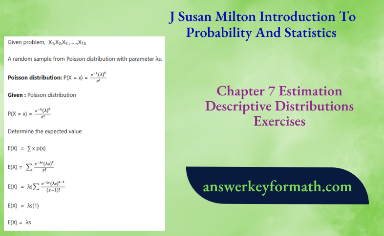
Given problem statement, X is the number of paint defects in a square yard section of car body painted by robot.

A random sample from Poisson distribution with parameter λs.

Poisson distribution: P(X = x) = \(\frac{e^{-\lambda}(\lambda)^x}{x !}\)

Given : The random variable X is the number of paint defects in a square yard section of car body painted by robot.

Also X is the Poisson distribution with parameter λs.

Find the unbiased estimate for λs

Hence, the sample mean is the unbiased estimator of the population mean.

Then the estimator is

\(\hat{\mu}=\bar{X}\)  ,\(\widehat{\lambda s}=\bar{X}\)

Therefore, an unbiased estimator for λs \(\hat{\mu}=\bar{X}\) ,\(\widehat{\lambda s}=\bar{X}\)

J. Susan Milton Estimation Chapter 7 Descriptive Distributions Answers Page 221 Exercise 3  Problem 4

Given problem statement,X is the number of paint defects in a square yard section of car body painted by robot.

A random sample from Poisson distribution with parameter λs.

Determine the unbiased estimate for the average number of flaws per square yard.

Given: The random variable X is the number of paint defects in a square yard section of car body painted by robot.

Also X is the Poisson distribution with parameter λs.

Find the unbiased estimate for λs

Hence, the sample mean is the unbiased estimator of the population mean. Then the estimator is

\(\hat{\mu}=\bar{X}\), \(\widehat{\lambda s}=\bar{X}\)

Determine the unbiased estimate for the average number of flaws per square yard is

Σ_iX_i = 8 + 0 + 2 + 5 + 3 + 7 + 0 + 1 + 9 + 10 + 12 + 6 = 63

λ₈ = \(\frac{63}{12}\)

λ₈ = 5.25
​
Therefore, the unbiased estimate for the average number of flaws per square yard is, 5.25

J.Susan Milton Introduction To Probability And Statistics Principles And Applications Chapter 7 Page 221  Exercise 3  Problem  5

Given problem statement,X is the number of paint defects in a square yard section of car body painted by robot.

A random sample from Poisson distribution with parameter λs.

Determine the unbiased estimate for the average number of flaws per square foot.

​Initally,Determine the unbiased estimate for the average number of flaws per square yard is
​

Σ_iX_i = 8 + 0 + 2 + 5 + 3 + 7 + 0 + 1 + 9 + 10 + 12 + 6 = 63

​λ₈ = \(\frac{63}{12}\)

​λ₈ = 5.25

Determine the unbiased estimate for the average number of flaws per square foot is

One yard = Three feet

Hence, unbiased estimate

5.25 ×  3 = 15.75

Therefore, the unbiased estimate for the average number of flaws per square foot is 15.75

Solutions To Estimation And Descriptive Distributions Exercises Chapter 7 Milton Page 221  Exercise 4  Problem  6

Given problem statement,X is the number of requests for the system received per hour.

A random sample from Poisson distribution with parameter λs.

Poisson distribution: P(X = x) = \(\frac{e^{-\lambda}(\lambda)^x}{x !}\)

Given : The random variable X is the number of requests for the system received per hour.

Also X is the Poisson distribution with parameter λs.

Find the unbiased estimate for λs

Hence, the sample mean is the unbiased estimator of the population mean.

Then the estimator is  \(\hat{\mu}=\bar{X}\), \(\widehat{\lambda s}=\bar{X}\)

J.Susan Milton Introduction To Probability And Statistics Principles And Applications Chapter 7 ​Page 221  Exercise 4  Problem  7

Given problem statement,X is the number of requests for the system received per hour.

A random sample from Poisson distribution with parameter λs.

Determine the unbiased estimate for the average number of request received per hour.

Given : The random variable X is the number of requests for the system received per hour.

Also X is the Poisson distribution with parameter λs.

Find the unbiased estimate for λs

Hence, the sample mean is the unbiased estimator of the population mean. Then the estimator is

\(\hat{\mu}=\bar{X}\) , \(\widehat{\lambda s}=\bar{X}\)

Determine the unbiased estimate for the average number of requests received per hour is

 Σ_iX_i = 25 + 30 + 10 + 20 + 24 + 23 + 20 + 15 + 4 = 171

λ₈ = \(\frac{171}{9}\)

λ₈ = 19

​Therefore, the unbiased estimate for the average number of flaws per square yard is 19.

Chapter 7 Estimation And Distributions Examples And Answers Susan Milton ​Page 221  Exercise 4  Problem  8

Given problem statement,X is the number of requests for the system received per hour.

A random sample from Poisson distribution with parameter λs.

Determine the unbiased estimate for the average number of request received per quarter hour.

Determine the unbiased estimate for the average number of requests received per hour is
​
 Σ_iX_i  = 25 + 30 + 10 + 20 + 24 + 23 + 20 + 15 + 4 = 171

λ8 = \(\frac{171}{9}\)

λ8 = 19

Determine the unbiased estimate for the average number of requests received per quarter hour is

1hour = 60minutes

45 Minutes = \(\frac{45}{60}\) hour

Hence, unbiased estimate is

19 × \(\frac{45}{60}\)

= 14.25

Therefore, the unbiased estimate for the average number of requests received per quarter hour is,14.25

J.Susan Milton Introduction To Probability And Statistics Principles And Applications Chapter 7 Page 222  Exercise 5  Problem  9

Given problem statement,X is the distance in inches from the anchored end of rod to the crack location.

A random sample from binomial distribution with interval (0,b).

Determine the unbiased estimator for the average distance.

Given: The random samples X defines the distance in inches from the anchored end of rod to the crack location.

Also X follows the binomial distribution with interval(0,b).

Hence, the sample mean value is the unbiased estimator for the population mean.

Find the unbiased estimator for the average distance \(\hat{\mu}=\bar{X}\)

Therefore, the unbiased estimator for the average distance in inches from the anchored end of rod to the crack location is \(\hat{\mu}=\bar{X}\)

Probability And Statistics J. Susan Milton Chapter 7 Solved Step-By-Step Page 222  Exercise 5  Problem 10

Given problem statement is the distance in inches from the anchored end of rod to the crack location.

A random sample from binomial distribution with interval (0,b).

Next determine the estimate for p at approximately.

Given: The random samples X defines the distance in inches from the anchored end of rod to the crack location..

Also X follows the binomial distribution with interval (0,b).

Hence, the sample mean value is the unbiased estimator for the population mean.

Find the unbiased estimator for the average distance \(\hat{\mu}=\bar{X}\)

Determine the variance for X is s²

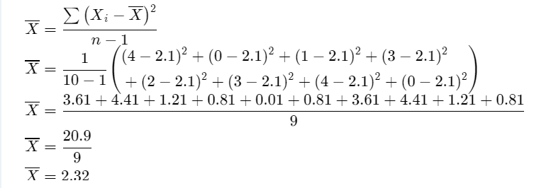
s² \(=\frac{\sum\left(X_i-\bar{X}\right)^2}{n-1}\)

s² =  \(\frac{1}{10 – 1}\)  (​(10−9.7)2+(8−9.7)2+(7−9.7)² + (9−9.7)² + (11−9.7)² + (10−9.7)² + (12−9.7)² +(9−9.7)² + (8−9.7)² +(13−9.7)²)

s²  =\(\frac{0.09+2.89+7.29+0.49+1.69+0.09+5.29+0.49+2.89+10.89}{9}\)

​s² = \(\frac{32.1}{9}\)

s² = 3.567
​

Therefore, an estimate for p based on the given data it is approximately 3.567.

J.Susan Milton Introduction To Probability And Statistics Principles And Applications Chapter 7 Page 222  Exercise 5  Problem 11

Given problem statement,X is the distance in inches from the anchored end of rod to the crack location.

A random sample from binomial distribution with interval (0,b).

Next determine the estimate for b.

Given: The random samples X defines the distance in inches from the anchored end of rod to the crack location..

Also X follows the binomial distribution with interval(0,b).

Hence, the sample mean value is the unbiased estimator for the population mean.

Find the unbiased estimator for the average distance \(\hat{\mu}=\bar{X}\)

Equating \(\bar{X}\) and E(x)

\(\frac{b}{2}\) = 9.7

b = 9.7 × 2

b = 19.4

Therefore, an estimate for b based on the given data is 19.4.

Online Help For J. Susan Milton Estimation Chapter 7 Exercises Page 222  Exercise 6  Problem 12

Given problem statement, showS is not unbiased estimator for σ.

Assume that E(S)=σ and using the contradiction method to show that S is not unbiased estimator for σ.

Given: Hence, the sample variance value is the unbiased estimator for the population variance.

Show that S is not unbiased estimator

E(S)= σ²

Assume,E(S) = σ

Based on theorem 3.3.2

V(X) = E(X²) −(E(X))²

Hence

​V(S)=E(S²) − (E(S))²

V(S) = σ² − σ²

V(S) = 0
​
Therefore,S is not unbiased estimator for σ because the variance value is zero.

J.Susan Milton Introduction To Probability And Statistics Principles And Applications Chapter 7 Page 222  Exercise 7  Problem 13

Given problem statement, k independent random samples and it generates unbiased estimators for the mean value.

Just show that the arithmetic average is an unbiased for μ.

So proof \(E\left(\frac{\bar{X}_1+\bar{X}_2+\ldots+\bar{X}_k}{k}\right)=\mu\)

Given: show that arithmetic average of the estimator is unbiased for μ.

Prove that  \(E\left(\frac{\bar{X}_1+\bar{X}_2+\ldots+\bar{X}_k}{k}\right)=\mu\)

Mean value of the estimator is, E[X_i] =  μ

Therefore, the arithmetic average of the estimator \(E\left(\frac{\bar{X}_1+\bar{X}_2+\ldots+\bar{X}_k}{k}\right)=\mu\) is an unbiased forμ and its proved.

Step-By-Step Guide To Estimation Exercises Chapter 7 Milton Page 222  Exercise 7  Problem 14

_iGiven problem:

\(\bar{X}\) = 0.8, n₁ = 9

\(\bar{X}\) = 0.95, n₂ = 3

\(\bar{X}\) = 0.7, n₃ = 200

Using previous value, for determine the averaging of three values to get the unbiased estimator for μ.

On previous lesson, the arithmetic average of the estimator is unbiased for μ.

Given:

\(\bar{X}\) = 0.8, n₁ = 9

\(\bar{X}\) = 0.95, n₂ = 3

\(\bar{X}\) = 0.7, n₃ = 200

Determine average of three values

⇒ \(\widehat{\mu}=\frac{\bar{X}_1+\bar{X}_2+\bar{X}_3}{3}\)

⇒  \(\widehat{\mu}=\frac{0.8+0.95+0.7}{3}\)

⇒  \(\widehat{\mu}=\frac{2.45}{3}\)

⇒  \(\widehat{\mu}\) = 0.8167

Therefore, Averaging the three values to get the estimate for μ is 0.8167.

J.Susan Milton Introduction To Probability And Statistics Principles And Applications Chapter 7 Page 222  Exercise 7  Problem 15

Given problem: \(=\frac{n_1 X_1+n_2 X_2+\ldots+n_k X_k}{n_1+n_2+\ldots+n_k}\)

Just show that given is an un biased for μ .so proof, E(\(\widehat{\mu_w}\)) = μ

Given: \(=\frac{n_1 X_1+n_2 X_2+\ldots+n_k X_k}{n_1+n_2+\ldots+n_k}\)

Then prove , E(\(\widehat{\mu_w}\)) = μ

Therefore, given \(\widehat{\mu_w}\) Is ann unbiased estimator for μ and its proved

Exercise Solutions For Chapter 7 Susan Milton Estimation And Distributions Page 222  Exercise 7  Problem 16

Previous problem: \(\widehat{\mu_w}\) = \(=\frac{n_1 X_1+n_2 X_2+\ldots+n_k X_k}{n_1+n_2+\ldots+n_k}\)

Using previous problem data and next deterine the estimate for based on the previous problem.

Given: \(=\frac{n_1 X_1+n_2 X_2+\ldots+n_k X_k}{n_1+n_2+\ldots+n_k}\)

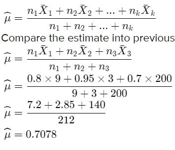
Therefore compared to the previous problem then the weighted average mean is less than mean.

J.Susan Milton Introduction To Probability And Statistics Principles And Applications Chapter 7 Page 223  Exercise 8  Problem 17

Given problem statement,X defines the number of heads obtained when a coin is tossed four times.

Determine the expected value E[X] and variance Var[X] for the variable X.

Given: The random variable X defines the number of heads obtained when a coin is tossed four times.

Also X follows the binomial distribution with parameters

n = 4

p = \(\frac{1}{2}\)

Determine the expected value

​​E[X] = np

E[X]= 4 × \(\frac{1}{2}\)

E[X] = 2

​Find the variance
​
​Var[X] = np(1 − p)

Var[X] = 4 × \(\frac{1}{2}\) (1−\(\frac{1}{2}\))

​Var[X]= 4 ×\(\frac{1}{2}\) × \(\frac{1}{2}\)

Var[X] = 1

​Therefore, the expected value and variance for the variable X is Expected Value: E[X] = 2,  Variance: Var[X] = 1

Page 223  Exercise 8  Problem 18

Given problem statement,X defines the number of heads obtained when a coin is tossed.

The number of heads obtained at 10 times. That means X = 10 and binomial distribution with parameters

n = 4

p = \(\frac{1}{2}\)

Given: The random variableX defines the number of heads obtained when a coin is tossed four times.

Also X follows the binomial distribution with parameters,

n = 4

p = \(\frac{1}{2}\)

When heads obtained at ten times.

That means X = 10 and apply all values in the binomial distribution formula

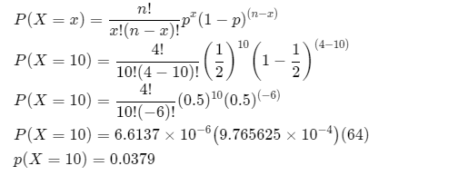
Therefore, the probability for obtain the number of heads at 10  times, 0.0379.

J.Susan Milton Introduction To Probability And Statistics Principles And Applications Chapter 7 Page 223  Exercise 8  Problem 19

Given problem statement,X defines the number of heads obtained when a coin is tossed.

Determine the expected value E[X] and variance Var[X]
for based on 10 observations of the variable X.

Given: The random variable defines the number of heads obtained when a coin tossed.

That means [X = 10] and binomial distribution with parameters

n = 4

p = \(\frac{1}{2}\)

The mean and variance was given
​
​E[X] = 2

Var[X] = 1

​Then determine the mean and variance for ten observations.

Mean is summation of all observations divided by number of observations.

The means value is 2.

Variance is sum of squares of each observation subtracted by the mean.

Hence, the variance value is 1

Therefore, based on 10 observations the expected value and variance for the variable X is  Expected Value: E[X] = 2 Variance: Var[X] = 1

Page 223  Exercise 8  Problem 20

Given problem statement, X defines the number of heads obtained when a coin is tossed.

The variance Var[X] of the variable X is an unbiased estimate for s².

Next determine the variance of the value \(\bar{X}\)

Given: The random variable defines the number of heads obtained when a coin tossed.

Apply n = 10 for the observations

The unbiased estimate for the variance of X is s².

Then the \(\bar{X}\)

J.Susan Milton Introduction To Probability And Statistics Principles And Applications Chapter 7 Page 223  Exercise 9  Problem 21

Given: The Random Samples are X₁,X₂,X₃ ,…..,Xn with mean and variance.

Using mean μ and the variance σ²

Value for prove that the below function

Given: The Random Samples are X₁,X₂,X₃ ,…..,X_n with mean μ and variance σ².

Prove that \(\frac{\sum\left(X_i-\bar{X}\right)^2}{n}=\frac{(n-1) s^2}{n}\) and  E(s² ) = σ²

Consider LHS

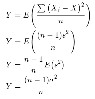
Therefore, the Random Samples X₁,X₂,X₃ ,…..,X_n with mean μ Value and variance σ²  Value for \(\frac{\sum\left(X_i-\bar{X}\right)^2}{n}=\frac{(n-1) s^2}{n}\) and its proved

Page 223  Exercise 10  Problem 22

Given: The Random Sample  X₁,X₂,X₃ ,…..,X_m  with size m and parameter n.

Using method of moments technique to Determine the first moment of the given sample.

Given: The Random Sample X₁,X₂,X₃ ,…..,X_m with size m and parameter n.

Also, it follows the Binomial Distribution X₁,X₂,X₃ ,…..,Xm

Use method of moments to find the estimator for p,

M₁ = \(\frac{\sum_i X_i}{m}=\bar{X}\)

Find the first moment of the sample, E(X) = np

Therefore, using Method of Moments technique for find the estimator of p is \(\hat{p}=\frac{\bar{X}}{n}\) and its proved.

J.Susan Milton Introduction To Probability And Statistics Principles And Applications Chapter 6 Descriptive Distributions

Introduction To Probability And Statistics Chapter 6 Exercises Solutions  Page 192  Exercise 1  Problem 1

In this case a statistical study is appropriate.

The population of interest is consisted of the wind speed per day.

An engineer can measure the speed over some period of time and then determine various statistics of that sample including

1. Mean

2. Minimal

3. Maximal value

4. Sample deviance etc..

The draw necessary conclusions about the population based on observing the given sample.

Thus, In this case, a statistical study is appropriate because of various statistics of that sample including Mean, Minimal, maximal value, sample deviance, etc. Hence, the maximum wind speed per day at all sites can be designed.

Read and Learn More J Susan Milton Introduction To Probability And Statistics Solutions

J.Susan Milton Introduction To Probability And Statistics Principles And Applications Chapter 6 Page 192  Exercise 2  Problem 2

In this case study:

A statistical study is appropriate. Because the population of interest is consisted of two groups of cuttings:

1. A control group

2. A test group

Various static test can be used for this kind of problem to determine whether or not there is a statistical significant between group or in this case whether or not indoleacetic acid really is effective.

Thus, the botanist thinks that indoleacetic acid is effective in stimulating the formation of roots in cutting from the lemon tree.

Solutions To Descriptive Distributions Exercises Chapter 6 Susan Milton Page 192  Exercise 3  Problem 3

In this case study:

A statistical study is not appropriate.

Because the sample might be too small to correctly approximate the average time and cost required to complete the job.

Thus, an architectural firm is to sublet a contract for a wiring project.

Chapter 6 Descriptive Distributions Examples And Answers Susan Milton Page 192  Exercise 4  Problem 4

In this case study:

A statistical study is not appropriate. Because the length of the sessions does not tell us anything about the occupancy of the terminal.

Thus, A statistical study is not appropriate in a computer system that has a number of remote terminals attached to it. Because the length of the sessions does not tell us anything about the occupancy of the terminal.

J.Susan Milton Introduction To Probability And Statistics Principles And Applications Chapter 6 Page 192  Exercise 5  Problem 5

In this case study:

A statistical study is appropriate.

Because the population of interest is consisted of the affected workers. We can also draw a random sample out of those 50000 workers, because the original population might be too large to study in its entirety.

Sampling the people from population would help us draw necessary conclusion about the population.

Thus, the statistical study is appropriate. Because the population of interest consists of the affected workers. prior to changing from the traditional is appropriate and also drew a random sample out of those 50,000 workers, because the original population might be too large to study entirety.

Probability And Statistics J. Susan Milton Chapter 6 solved Step-By-Step Page 192  Exercise 6  Problem 6

Frist we need to find the random variable.

Then identify with know or unknown mean.

Given:

Random variable  = X₁

Particular level =  24 hours period.

Now , Let X₁  be the random variable for the particular level for the first 24-hour period.

The random variable is normally distributed with unknown mean μ and also unknown variance is σ, so that we get  X₁ ≈ N(μ,σ²)

Thus, the distribution of this random variable is  X₁ ≈ N(μ,σ²).

J.Susan Milton Introduction To Probability And Statistics Principles And Applications Chapter 6 Page 192  Exercise 6  Problem 7

Now apply the value in the equation:

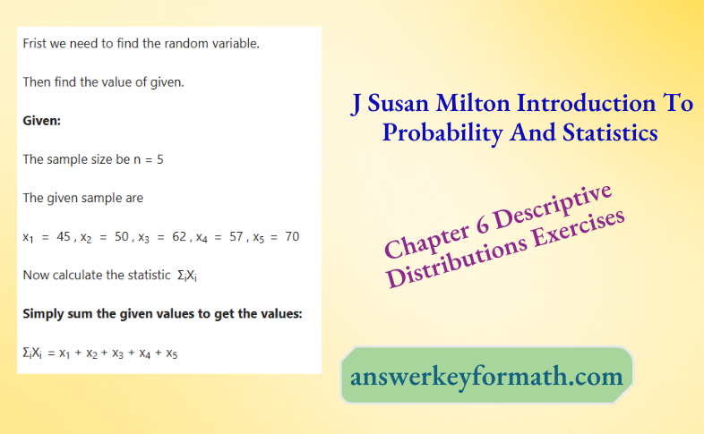
Σ_iX_i   = 45 + 50 + 62 + 57 + 70

Σ_iX_i  = 284

The sample size be n = 5

The given sample are

x₁  =  45 , x₂  =  50 , x₃  =  62 , x₄  =  57 , x₅  =  70

Now calculate the statistic Σ_iX_i/n

Simply sum the given values to get the values:

 _ΣiX²i    = x²₁ + x²₂ + x²₃ + x²₄ + x²₅

Now apply the value in the equation

Σ_iX²_i  = 45² + 50² + 62² + 57² + 70²

Σ_iX²_i  = 16518

The sample size be n = 5

The given sample are

x₁  =  45 , x₂  =  50 , x₃  =  62 , x₄  =  57 , x₅  =  70

Now calculate the statistic  Σ_iX²_i 

Simply sum the given values to get the values:

\(\Sigma_i \frac{X_i}{n}=\frac{x_1+x_2+x_3+x_4+x_5}{n}\)

Now apply the value in the equation

\(\Sigma_i \frac{X_i}{n}=\frac{45+50+62+57+70}{5}\)

⇒  \(\Sigma_i \frac{X_i}{n}\) = 56. 8

Now we going to calculate the statistic max_i {X_i},so that we to find the biggest value from the given sample.

By looking the values, we can easily identify them max_i {X_i}= x₅ = 70.

Now we going to calculate the statistic min_i {X_i}, so that we to find the biggest value from the given sample.

By looking the values, we can easily identify them min_i {X_i} = x₁ = 45.

Thus, the random variable value is Σ_iX_i  = 284

 Σ_iX_i =  16518

\(\Sigma_i \frac{X_i}{n}\) =   56.8

Max_i {X_i}= x₅ = 70.

Min_i {X_i} = x₁ = 45.

J.Susan Milton Introduction To Probability And Statistics Principles And Applications Chapter 6 Page 192  Exercise 6  Problem 8

Frist we need to find the random variable.

Then find the value of given.

The sample size be n = 5

The given sample are

x₁  =  45 , x₂  =  50 , x₃  =  62 , x₄  =  57 , x₅  =  70

The random variables X5and \(\frac{X_5-\mu}{\sigma}\) are not a statistic.

Since this random variable we can’t determine its numerical value from a random sample.

Thus, this random variable we can’t determine its numerical value from a random sample.

Page 193  Exercise 7  Problem 9

Given:

The number is = 02,03,04,05,06,07

First, we need to find the length of the categories.

To construct a Stem and leaf diagram, we have to use the initial two digits as stems, in this case 02,03,04,05,06,07

The third digit will be representation a leaf.

By applying the logic to the given sample, so we get that easily construct the given stem and leaf diagram:

02 ∣ 0

03 ∣ 079909

04 ∣ 407549262

05 ∣ 75012268431

06 ∣ 1612120

07 ∣ 0

Thus, the construct Stem and leaf diagram. By applying the logic to the given sample, so we get that easily construct the given stem and leaf diagram:

02 ∣ 0

03 ∣ 079909

04 ∣ 407549262

05 ∣ 75012268431

06 ∣ 1612120

07 ∣ 0

Online Help For J. Susan Milton Descriptive Distributions Chapter 6 Exercises Page 193  Exercise 7  Problem 10

By turning the stem and leaf diagram to the side , we can very clearly see that the diagram has a notorious bell shape, thus confirming the persons suspicious of it being normally distributed.

Hence we should not be surprised if we hear someone claim such thing.

J.Susan Milton Introduction To Probability And Statistics Principles And Applications Chapter 6 Page 193  Exercise 7  Problem 11

First we need to find the biggest value.

Then we are going to find the smallest value.

Given:

First half unit = \(\frac{1}{1000}\)

Other Half unit= .0005

To break the given data into six category , first we have to find the length of the interval convering the data.

The biggest value from the sample which is 0.070

The smallest value from the sample which is 0.020

0.070 − 0.050  =  0.020

To find the length of the categories for that we going to divide the length of the whole interval by the number of categories.

Now, Split data into 6 categories and we calculate the length of 0.02 units.

To divide those number and round it up to the nearest number that has the same number of decimals as the original data.

\(\frac{0.02}{6}\) = 0.00333333

The data has three decimals, so we going to round the calculated number to 0.010.

Hence the length of each category.

The lower boundary for the first category is obtained by subtracting 0.0005 from the lowest value of the sample which is 0.02.

0.02 − 0.0005 = 0.0195

Hence the lower boundary for the first category is 0.0195.

To find the remaining categories, we have to successively add the length of each category starting from the lowest boundary, which is 16.25.

0.0195 + 0.010 = 0.0295 ⇒ [0.0195,0.0295⟩

0.0295 + 0.010 = 0.0395 ⇒ [0.0295,0.0395⟩

0.0395 + 0.010 = 0.0495 ⇒ [0.0395,0.0495⟩

0.0495 + 0.010 = 0.0595 ⇒ [0.0495,0.0595⟩

0.0595 + 0.010 = 0.0695 ⇒ [0.0595,0.0695⟩

0.0695 + 0.010 = 0.0795​ ⇒ [0.0695,0.0795⟩

Thus, the method outlined in this section breaks these data into six categories and also add the length of each category starting from the lowest boundary, which is 16.25

0.0195 + 0.010 = 0.0295 ⇒ [0.0195,0.0295⟩

0.0295 + 0.010 = 0.0395 ⇒ [0.0295,0.0395⟩

0.0395 + 0.010 = 0.0495 ⇒ [0.0395,0.0495⟩

0.0495 + 0.010 = 0.0595 ⇒ [0.0495,0.0595⟩

0.0595 + 0.010 = 0.0695 ⇒ [0.0595,0.0695⟩

0.0695 + 0.010 = 0.0795​ ⇒ [0.0695,0.0795⟩

Step-By-Step Guide To Descriptive Distributions Exercises Chapter 6 Milton Page 193  Exercise 8  Problem 12

Since the stem and leaf diagram is slightly skewed to the left instead of having a normal bell shape it can be suggested that the data comes from a family of X₂ distribution.

Thus, the stem and leaf diagram is slightly skewed to the left instead of having a normal bell shape.

J.Susan Milton Introduction To Probability And Statistics Principles And Applications Chapter 6 Page 193  Exercise 9   Problem 13

Given:

The number is = 5,6,7,8,9,10

First, we need to find the length of the categories and then find the value.

Now

To construct Stem and leaf diagram, we have to use initial digits as “stems”, in this case 5,6,7,8,9,10

The second digits will be representation a leaf.

By applying the logic to the given sample, so we get that easily construct the given stem and leaf diagram:

5 ∣ 3

6 ∣ 12728257

7 ∣ 6467816399117494

8 ∣ 8728710275241

9 ∣ 056127563

10 ∣ 0

Thus, the construct for the Stem and leaf diagram is given below:

5 ∣ 3

6 ∣ 12728257

7 ∣ 6467816399117494

8 ∣ 8728710275241

9 ∣ 056127563

10 ∣ 0

J.Susan Milton Introduction To Probability And Statistics Principles And Applications Chapter 6 Page 193  Exercise 9  Problem 14

To construct Stem and leaf diagram, we have to use initial digits as “stems”, in this case, 5,6,7,8,9,10

The second digit will be a representation a leaf.

By applying the logic to the given sample, so we get easily construct the given stem and leaf diagram:

​5 ∣ 3

​6 ∣ 12728257

7 ∣ 6467816399117494

8 ∣ 8728710275241

9 ∣ 056127563

10 ∣ 0

By turning this stem and leaf diagram to the side, we can very clearly see that the diagram has a notorious bell shape, thus confirming the assumption of it being normally distributed.

Thus, the assumption X is normally distributed. The given stem and leaf diagram is

5 ∣ 3

6 ∣ 12728257

7 ∣ 6467816399117494

8 ∣ 8728710275241

9 ∣ 056127563

10 ∣ 0

Exercise Solutions For Chapter 6 Susan Milton Descriptive Distributions Page 194  Exercise  10  Problem 15

Given:

The number is = 0,1,2,3,4,5

First, we need to find the length of the categories and then find the value.

Now

To construct Stem and leaf diagram, we have to use initial digits as “stems”, in this case 0,1,2,3,4,5

The second digits will be representation a leaf.

By applying the logic to the given sample, so we get that easily construct the given stem and leaf diagram:

0 ∣ 578

1 ∣ 19358620972988457

2 ∣ 06443483575730231

3 ∣ 6281007541

4 ∣ 05

5 ∣ 0

Thus, the construct for Stem and leaf diagram is given below:

0 ∣ 578

1 ∣ 19358620972988457

2 ∣ 06443483575730231

3 ∣ 6281007541

4 ∣ 05

5 ∣ 0

J.Susan Milton Introduction To Probability And Statistics Principles And Applications Chapter 6 Page 194  Exercise 10  Problem 16

Given:

The assumption that X is not normally distributed.

There might be a slight reason that X is not normally distributed as by turning the stem and leaf diagram to the sight.

We can see that it does not exactly resemble perfect symmetrical bell shape like a normal distribution, but rather slightly skewed to the left.

Thus, we can be suspicious about the data not being normally distributed.

Thus, the assumption that X mis not normally distributed.

0 ∣ 578

1 ∣ 19358620972988457

2 ∣ 06443483575730231

3 ∣ 6281007541

4 ∣ 05

5 ∣ 0

Page 194   Exercise 10  Problem 17

First we need to find the biggest value.

Then we going to find the smallest value.

To break the given data into seven category , first we have to find the length of the interval covering the data.

The biggest value from the sample which is 5.0

The smallest value from the sample which is0.5

5.0 − 0.5 = 4.5

Whole interval by the number of categories.

Now

Split data into 7 categories and we calculate the length of 4.5 units.

To divide those number and round it up to the nearest number that has the same number of decimals as the original data.

\(\frac{4.5}{7}\) = 0.642857

The data has one decimals, so we going to round the calculated number to0.6.

Hence the length of each category.

The lower boundary for the first category is obtained by subtracting0.7

0.5−0.05 = 0.45

Hence the lower boundary for the first category is0.45.

To finding the remaining categories, we have to successively add the length of each category starting from the lowest boundary, which is n 0.45.

0.45 + 0.7 = 1.15 ⇒ [0.45,1.15⟩

1.15 + 0.7 = 1.85 ⇒ [1.15,1.85⟩

1.85+0.7 = 2.55 ⇒ [1.85,2.55⟩

2.55 + 0.7 = 3.25 ⇒ [2.55,3.25⟩

3.25 + 0.7 = 3.95 ⇒ [3.25,3.95⟩

3.95 + 0.7 = 4.65 ⇒ [3.95,4.65⟩

4.65 + 0.7 = 5.35 ⇒ [4.65,5.35⟩

J.Susan Milton Introduction To Probability And Statistics Principles And Applications Chapter 6 Page 194  Exercise 10  Problem 18

Given:

Let one variable be X

A random sample of 50 mosses yields under observation

First, we need to find the frequency table.

Then we going to find the histogram of data.

The frequency table constructed by observing and counting how many of the values from the sample are located inside of each of those six categories.

The table is:

The relative frequency histogram data

Thus, the looking the shape of the histogram, we can clearly see that it resembles the bell shapes, but is slightly skewed to the left, it is just like the stem and leaf.

Diagram we calculated easier. Hence having characteristics is not normal density.

The table is given below:

J.Susan Milton Introduction To Probability And Statistics Principles And Applications Chapter 6 Page 195  Exercise 11  Problem 19

Given:

The 25th, 50th,75th, and 100th percentiles for X

First, we need to find the point X value.

Then we going to find the binomial value.

The first quartile of a random variable X is a point p _0.25

Such that P(X < p _0.25) ≤ 0.25
​
P(X ≤ p_0.25) ≥ 0.25

Then we can write as: P(X < p_0.25) ≤ 0.25 and the first quartile of a random variable is P(X ≤ p_0.25) ≥ 0.25

Thus, the first quartile of a random variable X is P(X ≤ p_0.25) ≥ 0.25.

Page 195  Exercise 11  Problem 20

Given:

n = 20

p = 0.5

First we need to find the point X value .

Then we going to find the binomial value.

If X is binomial variable with n = 20 and p = 0.5, then its first quartile is obtained by using the definition, and table from appendix or a mathematical software such as R.

The first percentile of this distribution is p_0.25 = 8

P(X < 8) = P(X ≤ 7) = 0.132 ≤ 0.25

P(X ≤ 8) = 0.2517 ≥ 0.25

Thus, the first quartile of a random variable p_0.25 = 8.

J.Susan Milton Introduction To Probability And Statistics Principles And Applications Chapter 6 Page 195  Exercise 11  Problem 21

Given: \(\int_0^p e^{-x} d x\) = 0.25

First we need to find the point X value.

Then we going to find the binomial value

To calculate exponential random variables with β = 1,

We have to solve the given equation:

\(\int_0^p e^{-x} d x\) = 0.25

Let integrate the given equation:

\(\int_0^p e^{-x} d x\)= \(\left.\left(-e^{-x}\right)\right|_0 ^p\)

\(\int_0^p e^{-x} d x\)= \(-\left(e^{-p}-e^0\right)\)

Where e⁰= 1

\(\int_0^p e^{-x} d x\) = \(-\left(e^{-p}-1\right)\)

\(\int_0^p e^{-x} d x\)= \(1-e^{-p}\)  ……………………….. (1)

To solve equation(1) so that we get

1 − e − p = 0.25

⇔  0.75  =  e − p

⇔ ln 0.75 =  −p

⇔p  = −ln 0.75 ≈ 0.2877

Thus, the pointp value is  ⇔  p_0.25 = −ln0.75.

Page 195  Exercise 12  Problem 22

Given:

(Deciles.) The 10th,20th,30th,40th,50th,60th,70th,80th,90th,and100th

First, we need to find the point 40th deciles X value.

Then we going to find the binomial value.

The 4th decile of a random variable X is a point p_0.4

Such that P(X < p_0.4) ≤ 0.4

P (X ≤ p_0.4 ) ≥ 0.4

Then can write the fourth decile of the random variable as P(X ≤ p_0.4) ≥ 0.4

Thus, the 4th decile of random variable of a random variable X is P(X ≤ p_0.4) ≥ 0.4.

J.Susan Milton Introduction To Probability And Statistics Principles And Applications Chapter 6 Page 195  Exercise 12  Problem 23

Given: λ = 20

First we need to find the point X value

Then we going to find the Poisson value.

If X is Poisson random variable with λ = 20, then its first 6th decile is obtained by using the definition, and table from appendix or a mathematical software such as R.

The first percentile of this distribution is p _0.6= 11

P(X<11) = P(X ≤ 10) = 0.5830 ≤ 0.6

P(X ≤ 11) = 0.6968 ≥ 0.6

Thus, the 6th decile X value is p_0.6 = 11.

J.Susan Milton Introduction To Probability And Statistics Principles And Applications Chapter 6 Page 195  Exercise 13  Problem 24

First we need to find the point X value .

Then diagram the relative cumulative frequency.

The relative cumulative frequency ogive from the data :

By using projection method , approximate the first quartile for X by drawing the horizontal line at he height of 25 then add a perpendicular line.

That passes through the previously obtained point on the relative cumulative frequency ogive to read the approximate value for it.

The related graph is:

Thus, the approximate first quartile X value is p_0.25 = 0.0 415.

J.Susan Milton Introduction To Probability And Statistics Principles And Applications Chapter 6 Page 195  Exercise 13  Problem 25

First we need to find the point X value .

Then diagram the relative cumulative frequency.

The relative cumulative frequency ogive from the data :

By using projection method , approximate the first quartile for X by drawing the horizontal line at he height of 40 (it means 40%)then add a perpendicular line.

That passes through the previously obtained point on the relative cumulative frequency ogive to read the approximate value for it.

The related graph is:

Thus, the approximate fourth decile X value is p_0.4 = 7.7.

J. Susan Milton Introduction To Probability And Statistics Principles And Applications Chapter 4 Continuous Distributions

Introduction To Probability And Statistics Chapter 4 Exercises Solutions Page 127   Exercise 1  Problem 1

Given:

The function  f(x) = kx where 2 ≤ x ≤ 4

To find – The value of k

Method: The method here used is probability and continuous random variable.

The function f(x) = kx.

For, 2 ≤ x ≤ 4 variable.

Assume x = 3.

f(3) = 3k

Consider f(3) = 1 for the function f(x).

​1 = 3k

k = \(\frac{1}{3}\)

Hence, it is verified that the value of k is k = \(\frac{1}{3}\)

Read and Learn More J Susan Milton Introduction To Probability And Statistics Solutions

J. Susan Milton Introduction To Probability And Statistics Principles And Applications Chapter 4 Page 127  Exercise 1  Problem 2

​Given:

The function f(x) = kx

Where  2 ≤ x ≤ 4.

To find:

Find the value of probabilities of P(2.5 ≤ X ≤ 3).

Method: The method here used is probability and continuous random variable.

The function f(x) = kx where 2 ≤ x ≤ 4

Substitute x = 3

f(3) = 3k

The function of P[2.5≤X≤3]

Here, there is no function that occurs between the X = 2.5 and X = 3 X.

Hence, it is verified that the function f(x) is not possible for the values P(2.5 ≤ X ≤ 3).

J. Susan Milton Introduction To Probability And Statistics Principles And Applications Chapter 4  Page 127  Exercise 1  Problem 3

J. Susan Milton Chapter 4 Continuous Distributions Answers Page 127  Exercise 1  Problem 4

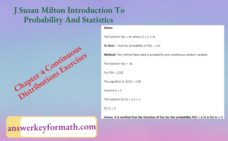
Given: 

The function f(x) = kx

where 2 ≤ x ≤ 4.

To find – Find the probability of P(2.5 < X ≤ 3)

Method: The method here used is probability and continuous random variable.

The function f(x) = kx

For P (2.5 < X ≤ 3)

The equation is, f(x) = 3k

Assume k = 2

The function

​f(x) = 3 × 2

f(x) = 6
​
Hence, it is verified that the function f(x) at P(2.5 < X ≤ 3) is f(x) = 6

J. Susan Milton Introduction To Probability And Statistics Principles And Applications Chapter 4 Page 128  Exercise 2  Problem 5

Given:

The function f(x) = \(\left(\frac{1}{10}\right) e^{\frac{-x}{10}}\)

To find – The function is a continuous random variable

Method : The method used is a probalility and continuous random variable

The given function f(x) =\(\left(\frac{1}{10}\right) e^{\frac{-x}{q p}}\)

Substitute 1 or x

f(1) \( = \frac{1}{10} e^{\frac{-x}{10}}\)

f(1)  =  0.0904

Hence, it is verified that the density of the function is f(1) = 0.0904

Solutions To Continuous Distributions Exercises Chapter 4 Susan Milton Page 128  Exercise 2  Problem 6

Given:

The function f(x)= \(\frac{1}{10} e^{\frac{-x}{10}}\)

To find –  Find the density at 7 minutes

Method: The method used here are probability and continuous random variable.

The given function

f(x) = \(\frac{1}{10} e^{\frac{-x}{10}}\)

For the density of 7 minutes

​f(7)  = \(\frac{1}{10} e^{\frac{-7}{10}}\)

f(7)  =  0.0496

Hence, it is verified that the density of the function at 7 minutes is f(7) = 0.0496

J. Susan Milton Introduction To Probability And Statistics Principles And Applications Chapter 4 Page 128  Exercise 2  Problem 7

Given:

The function f(x) = \(\frac{1}{10} e^{\frac{-x}{10}}\)

To find –  The probability of density of call last between 1 to 2 minutes.

Method: The method used here is probability and continuous random variable.

The given function is.

f(x) = \(\)

For the call last one minute

​f(1) = \(e^{\frac{-1}{10}}\)

​f(1) = 0.0904

For the call lasts two minutes

f(2) = 0.1 × \(e^{\frac{-2}{10}}\)

f(2) = 0.0607

The probaability of the call lasts one minuteto two minutes, the density of the function gradually increases to show the calls gain more and more density by increasing the call time.

Hence, it is verified that the call lasts from one to two minutes then the density of the call is also increasing.

J. Susan Milton Introduction To Probability And Statistics Principles And Applications Chapter 4 Page 128  Exercise 3  Problem 8

Given:

The graph of bird moving in θ.

To find –  The angle of the bird moving

Method: The method used in this problem is probability, continuous random variable, and graphical method.

Let the function f for the interval [0,2Π].

f(θ)\(=\int_0^{2 \Pi} \theta\)

Reduce the equation.

​f(θ) =  2Π − 0

f(θ) = 2Π
​
Hence, it is verified that the density of the function f with the interval [0,2Π] is f(θ) = 2Π

Chapter 4 Continuous Distributions Examples And Answers Susan Milton Page 128  Exercise 3  Problem 9

Given:

The graph of moving bird denoted in θ.

To find – Sketch the graph of the moving bird in uniform motion with interval [0,2Π].

Method: The method used in this problem is probability, continuous random variable, and graphical method.

The function of the moving bird in uniform distribution interval [0,2Π].

Let \(=\int_0^{2 \Pi} \theta\)

Reduce the equation.

​f(θ) = Π + Π

f(θ) = 2Π
​
The graph of the moving bird.

Hence, it is verified that the graph of a uniform distribution over the interval.

J. Susan Milton Introduction To Probability And Statistics Principles And Applications Chapter 4 Page 128  Exercise 3  Problem 10

Given:

The function f of moving bird in the angle θ.

To find – Sketch the graph of the function fin the interval [0,2Π].

Method: The method used in this problem is a probability, continuous random variable, and graphical method

Graph the function f and shade the orient within \(\frac{\Pi}{4}\)radians of home.

The graphs shows, the bird flying in the direction of \(\frac{\Pi}{4}\) radians from home in the straight direction from home.

Hence, it is verified that the 

J. Susan Milton Introduction To Probability And Statistics Principles And Applications Chapter 4 Page 128  Exercise 3  Problem 11

Given:

The function f mof the interval [0,2Π].

To find –  Find the probability of the function f with the orient within the
\(\frac{\Pi}{4}\) radians of home.

Method: The method used in this problem is a probability, continuous random variable, and graphical method.

The function for orient within the \(\frac{\Pi}{4}\) radians of the home .

​f(θ)\(  =\int_0^{2 \Pi} \theta+\frac{\Pi}{4}\)

Reduce the equation.

​f(θ) = \(2 \Pi+\frac{\Pi}{4}\)

​f(θ) = \(\frac{9 \Pi}{4}\)

Hence, it is verified that the possibilities of the moving bird within the
\(\frac{\Pi}{4}\) radians of home is \(=\frac{9 \Pi}{4}\)

Probability And Statistics J. Susan Milton Chapter 4 Solved Step-By-Step Page 129  Exercise 4  Problem 12

Given:

The graph of the probabilities.

To find: Show probabilities in terms of the cumulative distribution function F.

Method: The method used in this problem is a probability, continuous random variable, and cumulative distribution function.

The graph f(x) of the cumulative distribution function F(x) has the possible intervals of 0 ≤ x ≤ 20.

For graph A

F(x) = \(\int_0^{20} x+1 d x\)

Reduce the equation.

​F(x) = 20 + 1−(0 + 1)

F(x) = 20
​
The probability at graph A X≤ 5

Similarly, for the graph B, C, D, and E

​F(x)= \(\int_0^{20} x+1 d x\)

Reduce the equation

​F(x) = 20 + 1−(0 + 1)

F(x) = 20
​
The probability of graph B, X > 5.

The probability of graph C, X = 10.

The probability of graph D, 5 ≤ X < 10.

The probability of graph E, 5 < X < 10

Hence, it is verified.

The probability of the graph A, X ≤ 5.

The probability of the graph B, X > 5.

The probability of the graph C, X = 0.

The probability of the graph D, 5 ≤ X < 10.

The probability of the graph E, 5 < X < 10.

J. Susan Milton Introduction To Probability And Statistics Principles And Applications Chapter 4 Page 129  Exercise 5  Problem 13

Given:

The function f(x) = kx where 2 ≤ x ≤ 4.

To find –  Find the cumulative function of F(x).

Method:

The method used in this problem is a probability, continuous random variable, and cumulative distribution function.

The given function is f(x) = kx where 2 ≤ x ≤ 4.

The cumulative distribution function is

F(X) = \(\int_2^4(k x) d x\)

Reduce the equation.

​F(X) = 4k − 2k

F(X) = 0 2k
​
Hence, it is verified that the cumulative distribution function of F(x) = 2k.

Step-By-Step Guide To Continuous Distributions Exercises Chapter 4 Milton Page 129  Exercise 5  Problem 14

Given:

The cumulative distribution function , F(X) = \(=\int_2^4 k X d X\)

To find – Find the cumulative distribution function, P[2.5 ≤ X ≤ 3].

Method: The method used in this problem is a probability, continuous random variable, and cumulative distribution function.

The given function.

​F(X) = \(\int_2^4 k x d x\)

The cumulative distribution function for the interval P[2.5 ≤ X ≤ 3].

​F(X) = \(\int_{2.5}^3 k x \mathrm{dx}\)

Reduce the equation.

​F(X) = 3k − 2.5k

F(X) = 0.5k

Hence, it is verified that the cumulative distribution function of the interval P[2.5 ≤ X ≤ 3] is F(X) = 0.5k

J. Susan Milton Introduction To Probability And Statistics Principles And Applications Chapter 4 Page 129  Exercise 5  Problem 15

Given:

The function F with limits \(\lim _{n \rightarrow \infty} F(x)\) and \(\lim _{n \rightarrow \infty} F(x)\).

To find – Draw the graph of a function with limits \lim _{n \rightarrow \infty} F(x)

Method: The method used in this problem is a probability, continuous random variable, and cumulative distribution function.

The graph of the cumulative distribution function

Here, the graph of the function shows the function F is the increasing function.

This function is a non-decreasing function up to the interval \(\lim _{n \rightarrow \infty} F(x)\) and \(\lim _{n \rightarrow \infty} F(x)\) is possible in the graph of the function.

Hence, it is verified that graph of the cumulative distributive function Fand the function is non-decreasing.

J. Susan Milton Introduction To Probability And Statistics Principles And Applications Chapter 4 Page 129   Exercise 6  Problem 16

Given:

The function f(x) = \(\frac{1}{b-a}\)

To find – Find the uniform distribution over the interval (a,b).

Method: The method used in this problem is a probability, continuous random variable, and cumulative distribution function.

The function f(x) = \(\frac{1}{b-a}\)

The uniform distribution over the interval (a,b).

The cumulative distribution function

f(x) = \(\int_a^b \frac{1}{b-a} d x\)

f(x) = \(\left[\frac{x}{b-a}\right]_a^b\)

f(x) = \(\frac{b}{b-a}-\frac{a}{b-a}\)

f(x) = \(\frac{b-a}{b-a}\)

f(x) = 1

Hence, it is verified that the uniform distribution over the interval (a,b) is f(x)=1

Exercise Solutions For Chapter 4 Susan Milton Continuous Distributions Page 129  Exercise 7  Problem 17

Given: The function f(θ) \(=\int_0^{2 \Pi} \theta d \)

To find – 

Find the uniform distribution of f.

Method – The methods used here are a probability, cumulative random variable, and uniform distribution.

The function f(θ) \(=\int_0^{2 \Pi} \theta d \theta\)

For the cumulative distribution function, θ = Π.

f(θ) \(=\int_0^{2 \Pi} \theta d \theta\)

f(θ) = 2 Π

Hence, it is verified that the uniform distribution of cumulative function is f(θ) = 2Π.

J. Susan Milton Introduction To Probability And Statistics Principles And Applications Chapter 4 Page 129  Exercise 7  Problem 18

Given:

The function f(θ) = \(\int_0^{2 \Pi} \theta d \)

To find – Graph the function F and F is non-decreasing or not.

Method: The method used here is a probability, cumulative distributive function and uniform distribution.

The function.

f(θ) =  \(\int_0^{2 \Pi} \theta d \)

Reduce by uniform Distribution.

​F(θ) = [θ²]₀^2π

F(θ) = 4Π²

The graph of the function

Hence, it is verified that the uniform function is F(θ)=4Π2 and the function is non-decreasing. The graph of the function F

J. Susan Milton Introduction To Probability And Statistics Principles And Applications Chapter 4 Page 129   Exercise 8  Problem 19

Given:

The function f(x)=\(\frac{1}{10} e^{\frac{-x}{10}}\).

To find  – Find the Cumulative distribution f.

Method: The methods used here are probability, cumulative distribution function.

The function

f(x) = \(\frac{1}{10} e^{\frac{-x}{10}}\).

For the interval P[1 ≤ X ≤ 2] .

The cumulative distribution function X = 1

f(1) = \(\frac{1}{10} e^{\frac{-1}{10}}\)

f(1) = 0.906 × 0.1

f(1) = 0.906

The cumulative distribution function X = 2

​f(1) = \(\frac{1}{10} e^{\frac{-2}{10}}\)

f(2) = 0.1 × 0.818

f(2) = 0.0818
​
Hence, it is verified that the continuous random variable has only one possibilities of probability, but the cumulative distribution function has two probability values.

J. Susan Milton Introduction To Probability And Statistics Principles And Applications Chapter 4 Page 129  Exercise 9  Problem 20

Given:

The function f(x) = \(\frac{1}{\ln 2} \frac{1}{x}\).

To find – Find the cumulative distribution of function f.

Methods: The methods used here is the probability, cumulative distribution function

The given function f(x)= \(\frac{1}{\ln 2} \frac{1}{x}\)

The cumulative distribution of interval P[30 ≤ X ≤ 40].

For X = 30

f(x) = \(\frac{1}{\ln 2} \frac{1}{30}\)

f(x) = 1.44 × 0.33

f(x) = 0.475

Hence, it is verified that the cumulative distributive function of function f is f(x) = 0.475
​

J. Susan Milton Introduction To Probability And Statistics Principles And Applications Chapter 4 Page 129  Exercise 10  Problem 21

Given: The function

F(x) = \(\left\{\begin{array}{c}0, \mathrm{X}<-1 \\X+1,-1 \leq x \leq 0 \\1, x>0\end{array}\right.\)

To find – Find the cumulative distribution function.

Method: The methods used here are probability and cumulative distributive function.

The given function.

F(x) = \(\left\{\begin{array}{c}
0, \mathrm{X}<-1 \\
X+1,-1 \leq x \leq 0 \\
1, x>0
\end{array}\right.\)

The cumulative distribution function.

For, X < − 1.

F(x) = 0

For, −1 ≤ x ≤ 0.

F(x) = 1

For, x > 0.

F(x) = 1

Hence, it is verified that the cumulative distributive function is F(x)=1 and the function is non-decreasing for the limit \(\lim _{x \rightarrow-\infty} F(x)\) = 0 and \(\lim _{x \rightarrow-\infty} F(x)\) = 1.

J. Susan Milton Introduction To Probability And Statistics Principles And Applications Chapter 4 Page 129  Exercise 10  Problem 22

Given:

The function F(x)= \(\left\{\begin{aligned}
0, \mathrm{X} & \leq 0 \\
x^2, 0<x & \leq \frac{1}{2} \\
\frac{1}{2} x, \frac{1}{2}<x & \leq 0 \\
1, \mathrm{x} & >1
\end{aligned}\right.\)

​To find –  Find the cumulative distribution function.

Method: The methods used here are probability, cumulative distributive function.

The given function.

F(x) = \(\left\{\begin{array}{r}
0, \mathrm{X} \leq 0 \\
x^2, 0<x \leq \frac{1}{2} \\
\frac{1}{2} x, \frac{1}{2}<x \leq 0 \\
1, \mathrm{x}>1
\end{array}\right.\)

For, x ≤ 0.

F(x) =  0

For, 0 < x ≤ \(\frac{1}{2}\)

F(x) = \(\frac{1}{4}\)

For, \(\frac{1}{2}\) <x≤0.

F(x)= \(\frac{1}{4}\)

For, x > 1.

F(x) = 1

Hence, it is verified that the cumulative distributive function is F(x)= \(\frac{1}{4}\) and function is ono-decreasing with the limit F(x) = 0.

J. Susan Milton Introduction To Probability And Statistics Principles And Applications Chapter 4 Page 130  Exercise 11  Problem 23

Given:

The function f(x) = \(\frac{1}{6}\) (x) where 2 ≤ x ≤ 4.

To find – Find the function E(X) f(x) =\(\frac{1}{6}\)(x).

Method:

The method used here is probability, cumulative distributive function.

The function f(x)= \(\frac{1}{6}\)

The uniform distribution.

For, 2 ≤ x ≤ 4.

E(X) = \(\int_2^4 f(x) d x\)

Reduce the equation.

E(X) = \(\int_2^4 \frac{1}{6}(x) d x\)

E(X) = \(\frac{1}{6}\left[x^2\right]_2^4\)

E(X) =\(\frac{1}{6}\)(16 – 4)

E(X) = \(\frac{1}{6}\)(12)

E(X) = 2

Hence, it is verified that the uniform distribution of the function f(x) = \(\frac{1}{6}\) (x) E(x) = 2

J. Susan Milton Introduction To Probability And Statistics Principles And Applications Chapter 4 Page 130  Exercise 11  Problem 24

Given:

The function f(x) = \(\frac{1}{6}\) (x) where 2 ≤ x ≤ 4.

To find – 

Find E(X²).

Method: The methods used here are probability, Cumulative distributive function, and Uniform distribution.

The function f(x) = \(\frac{1}{6}\) (x).

The cumulative distribution of function.

E(X²) = \(\int_2^4(f(x))^2 d x\)

Reduce the equation.

​E(X²) = \(\int_2^4 \frac{1}{36}\left(x^2\right) d x\)

​E(X²) = ​\(\left.\frac{1}{36} \frac{x^3}{3}\right]_2^4\)

​E(X²) = \(\left(\frac{16}{27}\right)-\left(\frac{2}{27}\right)\)

Hence, it is verified the uniform distribution of the function f(x) = \(\frac{1}{6}x\) is ​E(X2) =\(\frac{14}{7}\).

Page 130  Exercise 12  Problem 25

Given:

The function f(x) = \(\frac{1}{10} e^{\frac{-x}{10}}\) where x>0.

To find – Find the moment generating function M​​X(t).

Method: The method used here is the cumulative distribution function and the uniform distribution.

The function f(x) = \(\frac{1}{10} e^{\frac{-x}{10}}\) where x>0

The expression for moment generating function M​X(t)

M​X(t)= E [ext]

Reduce the equation.

M​_x(t) = \(\int_1^{\infty} e^{t x} \frac{1}{10} e^{\frac{-x}{10}} d x\)

M​_x(t) = 0.1 [\(\left[e^{t x} \frac{1}{10} e^{\frac{-x}{10}}\right]_1^{\infty}\)

M​X(t) = 0.1 \(\left[e^{t x-\frac{x}{10}}\right]_1^{\infty}\)

M​_x(t) = 0.1 \(\left[e^{t-\frac{1}{10}}-e^{\infty}\right]\)

M​_x(t) = 0.1 \(0.1\left[e^{t-0.1}-\infty\right]\)

M​_x(t) = ∞

Hence, it is verified that the moment generating function is M​_x(t) = ∞.

J. Susan Milton Introduction To Probability And Statistics Principles And Applications Chapter 4 Page 130  Exercise 12  Problem 26

Given:

The function f(x)= \(\int_1^{\infty} e^{t x} \frac{1}{10} e^{\frac{-x}{10}} d x\) where x>0.

To find – Find the average length of such a call with the moment generating function.

Method: The method used here is the cumulative distribution function and the uniform distribution.

The function f(x)= \(\int_1^{\infty} e^{t x} \frac{1}{10} e^{\frac{-x}{10}} d x\).

The Expression for the moment generating function.

M​_x(t) = E[e^tX]

M​_x(t) = \(0.1\left[e^{t-\frac{1}{10}}-\infty\right]\)

For the average length of a call, assume t = 1.

M​_x(1) = \(0.1\left[e^{t-\frac{1}{10}}-\infty\right]\)

M​_x(t) = \(0.1\left[e^{t-\frac{1}{10}}-\infty\right]\)

M​_x(t) = ∞

Hence, it is verified that the average length of such a call in moment generating function is M​_x(t) = ∞.

Introduction To Probability And Statistics Principles And Applications Chapter 3 Discrete Distributions Exercises

Introduction To Probability And Statistics Chapter 3 Exercises Solutions Page 73  Exercise 1  Problem 1

We are asked to identify whether the given variable is discrete or not discrete.

Given that M as the number of meteorites hitting a satellite per day. It seems to be a count variable because it will take the value as 0,1,2…

Hence, the number of times a satellite gets hit by the meteorites is random and countable.

So M is a discrete random variable.

Therefore, we conclude that M is a discrete random variable as it holds the countable many values.

J. Susan Milton Discrete Distributions Chapter 3 Answers Page 73  Exercise 2  Problem 2

We are asked to identify whether the given variable is discrete or not discrete.

Given that N as the number of neutrons expelled per thermal neutron that is absorbed in the uranium fission−235.

This seems to be a count variable because it takes the value as 0,1,2…

Hence, the number of neutrons gets expelled is random and so N is a discrete random variable.

Therefore, we conclude that N is a discrete random variable as it holds the countable many values.

Read and Learn More J Susan Milton Introduction To Probability And Statistics Solutions

Introduction To Probability And Statistics Principles And Applications Chapter 3 Page 73  Exercise 3  Problem 3

We are asked to identify whether the given variable is discrete or not discrete.

Given that prompt neutrons holds for 99% of all emitted neutrons and are released within 10⁻⁴ of this fission.

Delayed neutrons are emitted for several hours.

Let us take D as the random variable which represents the time at which the emission of delayed neutron is continuous.

The feasible values of the random variable D will be the set of some intervals or continuous of real numbers.

Therefore, we conclude that the variableD is not discrete as the set of real numbers is neither finite nor countably infinite.

Solutions To Discrete Distributions Exercises Chapter 3 Susan Milton Page 74  Exercise 4  Problem 4

We are asked to identify whether the given variable is discrete or not discrete.

Given that the variable O is the random variable which represents the actual resistance of a bell selected at random.

From the given question we are able to understand that the value of O will be between 1.5 and 1.5.

Therefore, we conclude that the variable O is a continuous random variable as the value will be between 1.5 and 3.

Introduction To Probability And Statistics Principles And Applications Chapter 3 Page 74  Exercise 5  Problem 5

We are asked to identify whether the given variable is discrete or not discrete.

Given that the variable X denotes the number of power failures per month in the Tennessee Valley power network.

This seems to be a count variable since it holds the value 0,1,2,…

So it consists of a countable many values.

Therefore, we conclude that the variable X is a discrete random variable as the power failure will be happening at a random value.

Introduction To Probability And Statistics Principles And Applications Chapter 3 Page 74   Exercise 6  Problem6

Introduction To Probability And Statistics Principles And Applications Chapter 3 Page 74  Exercise 6  Problem 7

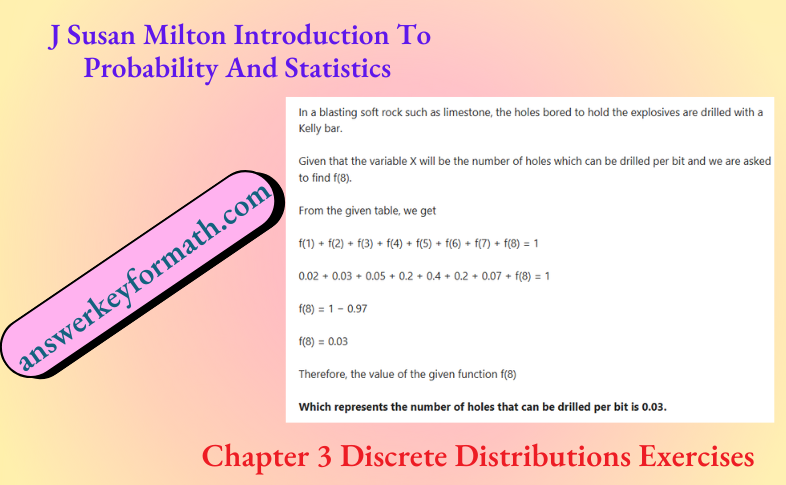
In a blasting soft rock such as limestone, the holes bored to hold the explosives are drilled with a Kelly bar.

Given that the variable X will be the number of holes which can be drilled per bit and we are asked to find the table for F.

For the values x = 1,2,3,4,5,6,7,8, the value of F(x) will be
​
​F(1) = P[X ≤ 1]

​F(1)  = f(1)

​F(1)  =0.02
​

​F(2) = P[ X≤2 ]

​F(2)  = f(1) + f(2)

​F(2) = 0.02+0.03

​F(2) = 0.05
​

​F(3) = P[X ≤ 3]

​F(3) = f(1)+ f(2) + f(3)

​F(3) = 0.02 + 0.03 + 0.05

​F(3) = 0.1
​

​F(4) = P[X ≤ 4]

​F(4) = f(1) + f(2) + f(3) + f(4)

​F(4) = 0.02 + 0.03 + 0.05 + 0.2

​F(4)  = 0.3
​
​F(5) = P[X ≤ 5]

​F(5) =f(1) + f(2) + f(3) + f(4) + f(5)

​F(5)= 0.02 + 0.03 + 0.05 + 0.2 + 0.4

​F(5) = 0.7
​
​F(6) = P[X ≤ 6]

​F(6) = f(1) + f(2) + f(3) + f(4) + f(5) + f(6)

​F(6) = 0.02 + 0.03 + 0.05 + 0.2 + 0.4 + 0.2

​F(6) = 0.9
​

​F(7) = P[X ≤ 7]

​F(7)  = f(1) + f(2) + f(3) + f(4) + f(5) + f(6) + f(7)

​F(7)  = 0.02 + 0.03 + 0.05 + 0.2 + 0.4 + 0.2 + 0.07

​F(7)  = 0.97
​

​F(8) = P[X ≤ 8]

​F(8)  = f(1) + f(2) + f(3) + f(4) + f(5) + f(6) + f(7) + f(8)

​F(8) = 0.02 + 0.03 + 0.05 + 0.2 + 0.4 + 0.2 + 0.07 + 0.03

​F(8)  = 1
​
Therefore, the table for the value F will be

Introduction To Probability And Statistics Principles And Applications Chapter 3 Page 74  Exercise 6  Problem 8

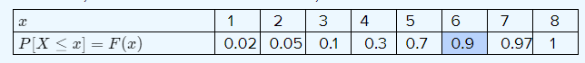
In a blasting soft rock such as limestone, the holes bored to hold the explosives are drilled with a Kelly bar.

Given that the variable X will be the number of holes which can be drilled per bit and we are asked to find out the probability that a bit can be used to drill between three and five holes inclusive.

Using the F table, we get the probability of drilling between three and five holes inclusive

​P [3 ≤ X ≤ 5] = P[X ≤ 5] − P[X > 3]

​P [3 ≤ X ≤ 5] = P[X ≤ 5]−P[X ≤ 2]

​P [3 ≤ X ≤ 5] = 0.7 − 0.05

​P [3 ≤ X ≤ 5]= 0.65
​
Therefore, by using the table F, we get the probability of drilling between three and five holes inclusive is 0.65.

Chapter 3 Discrete Distributions Examples And Answers Susan Milton Page 75  Exercise 7   Problem 9

Let X denote the number of computer systems operable at the time of the launch.

Assume that each system is operable is 0.9.

We have to use the tree of table to find the density table.

Obtain the density table by

From the table  sample space (S) is given below:

S={yyy,yyn,yny,ynn,nyy,nyn,nny,nnn}

Here, the probability of system is operable(y) is 0.9 and probability of system is not operable(n) is 0.1 =( 1−0.9).

Therefore, the probabilities are given below:

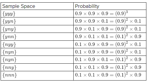
The density for X is given below

At x = 0, f(0) = (0.1)3

At x = 1

f(1) = (0.9)(0.1)² + (0.9)(0.1)² + (0.9)(0.1)²

f(1) =  (0.9)(0.1)² (1 + 1 + 1)

f(1) = 3(0.9)(0.1)²

At x = 2

f(2) = (0.1)(0.9)² + (0.1)(0.9)² + (0.1)(0.9)²

f(2) = (0.1)(0.9)² (1 + 1 + 1)

f(2) = 3(0.1)(0.9)²

At x = 3

f(3) = (0.9)³

The density table for X is given below

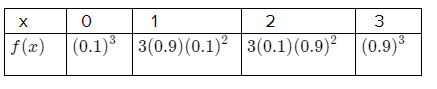
Hence the equation x ²+ 6x in the form of (x + k)² + his (x + 3)² − 9.

Introduction To Probability And Statistics Principles And Applications Chapter 3 Page 75  Exercise 7  Problem 10

Let X denote the number of computer systems operable at the time of the launch.

Assume that each system is operable is 0.9.

There is a pattern to the probabilities in the density table.

In particular f(x) = k(x)(0,9)x (0.1)3 − x

Where k(x) gives the number of paths through the tree yielding a particular value for X.

We have to use F to find the probability that at least one system is operable at launch time.

We have to find the value of P(x ≥ 1).

Consider

⇒  P(x ≥ 1)

= 1−P(x < 1)

=  1−P(x ≤ 0)

=  1 − F(0)

From F table, the value of F(0) is 0.001.

Therefore

⇒ P(x ≥ 1) 

= 1 − F(0)

= 1 − 0.001

= 0.999

Thus the probability that at least one system is operable at launch time is 0.999.

Hence using F table, the probability that at least one system is operable at launch time is 0.999.

Probability And Statistics J. Susan Milton Chapter 3 Solved Step-By-Step Page 75  Exercise 8  Problem 11

Given the function is

F(x) = \( \begin{cases}0 & x<0 \\ .70 & 0 \leq x<1 \\ .90 & 1 \leq x<2 \\ .95 & 2 \leq x<3 \\ .98 & 3 \leq x<4 \\ .99 & 4 \leq x<5 \\ 1.00 & x \geq 5\end{cases}\)

To draw the graph of this function.

Cumulative distribution

Let X be a discrete random variable with density f.

The cumulative distribution function for X, denoted by F is defined by F(x) = P[X≤x]for x real.

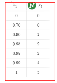
Yes. This function is called the step function.

Introduction To Probability And Statistics Principles And Applications Chapter 3 Page 75   Exercise 8  Problem 12

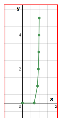
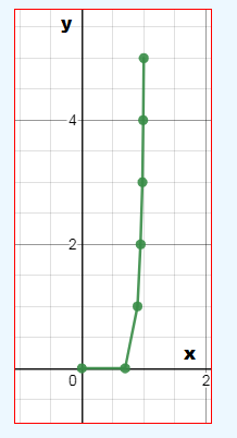
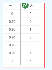
Given that

F(x) = \(\begin{cases}0 & x<0 \\ .70 & 0 \leq x<1 \\ .90 & 1 \leq x<2 \\ .95 & 2 \leq x<3 \\ .98 & 3 \leq x<4 \\ .99 & 4 \leq x<5 \\ 1.00 & x \geq 5\end{cases}\)

Need to determine that it is a continuous function

A function is said to be continuous as the values of x increases the function also increases.

Here I have attached an example graph which clearly explain that the function is continuous function.

Example of graph:

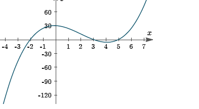
Similarly in our case also the graph increases as the value of x increases the function value also increases .

For example ,in our case consider any value to check that above said condition are satisfied.

1. f(a) Exists for any value of x

2. \(\lim _{x \rightarrow a} f(x)\) for each and every value of x from 0 to 5,the function exists.

3. \(\lim _{x \rightarrow a} f(x)\) = f(a) at last the function for every values

Therefore the given function is a continuous function.

Introduction To Probability And Statistics Principles And Applications Chapter 3 Page 75  Exercise 8  Problem 13

We need to find the \(\lim _{x \rightarrow \infty} F(x)\) and \(\lim _{x \rightarrow \infty}\) F(x)

Cumulative distribution

Let X be a discrete random variable with density f.

The cumulative distribution function for X, denoted by F, is defined by F(x) = P[X≤x] for x real.

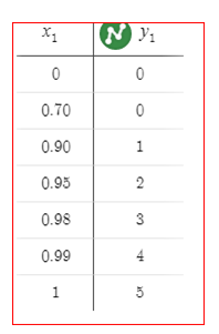
The value of \(\lim _{x \rightarrow \infty} \) F(x) = 1 and the value of \(\lim _{x \rightarrow \infty}\) F(x) = 0

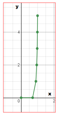
The value of \(\lim _{x \rightarrow \infty} \)F(x) = 1 and the value of \(\lim _{x \rightarrow \infty}\) F(x) = 0

Step-By-Step Guide To Discrete Distributions Exercises Chapter 3 Milton Page 76  Exercise  9  Problem 14

Given: In an experiment to graft Florida sweet orange trees to the root of a sour orange variety, a series of five trials is conducted.

Let X denote the number of grafts that fail.

The density for X is given in

To find –  Find E[X]

We can find the E[X] by the following formula

E[X] = \(\sum_z x f(x)\)

So the expectation of the random variable X wil be as foliows:
​
​E[X] = \(\sum_z x f(x)\)

​E[X]  = 0 × f(0) + 1 × f(1) + 2 × f(2) + 3 × f(3) + 4 × f(4) + 5 × f(5)

​E[X] = 0 × 0.7 + 1 × 0.2 + 2 × 0.05 + 3 × 0.03 + 4 × 0.01 + 5 × 0.01

​E[X] = 0 + 0.2 + 0.1 + 0.09 + 0.04 + 0.05

​E[X] = 0.48

​For the above two calculations we have used the R software.

Hence, from the above explanation value of E[X] is 0.48

Introduction To Probability And Statistics Principles And Applications Chapter 3 Page 76   Exercise 9  Problem 15

Given: In an experiment to graft Florida sweet orange trees to the root of a sour orange variety, a series of five trials is conducted.

Let X denote the number of grafts that fail.

The density for X is given in

TO find – Find μ_x

Since, we know that μ_x =  E[X]

Therefore;So the expectation of the random variable X wil be as foliows:

E[X]  = \(\sum_z x f(x)\)

E[X]  = 0 × f(0) + 1 × f(1) + 2 × f(2) + 3 × f(3) + 4 × f(4) + 5 × f(5)

E[X]  = 0 × 0.7 + 1 × 0.2 + 2 × 0.05 + 3 × 0.03 + 4 × 0.01 + 5 × 0.01

E[X]  = 0 + 0.2 + 0.1 + 0.09 + 0.04 + 0.05

E[X]  = 0.48

Hence, μ_x E[X] = 0.48

Hence, from the above explanation the value of μX is equal to 0.48.

Introduction To Probability And Statistics Principles And Applications Chapter 3 Page 76  Exercise 9   Problem 16

In an experiment to graft Florida sweet orange trees to the root of a sour orange variety, a series of five trials is conducted.

Let X denote the number of grafts that fail.

The density for X is  

To Find μ_x

We can find the E[X²] by the following formula

E[X²] = \(\sum_z x f(x)\)

So the expectation of the random variable x will be as follows:
​
​E[X²] =  \(\sum_z x f(x)\)

f(x) =0 × f(0)+ 1 × f(1) + 2² × f(2) + 32 × f(3) + 42× f(4) + 52 × f(5)

f(x) = 0 × 0.7 + 1 × 0.2 + 4 × 0.05 + 9 × 0.03 + 16 × 0.01 + 25 × 0.01

f(x) = 0.210.210.27 + 0.1610.25

f(x) = 1.08
​
For the above two calculations we have used the R software.

Hence, from the above explanation the value of E[X²] is equal to 1.08.

Introduction To Probability And Statistics Principles And Applications Chapter 3 Page 76   Exercise 9  Exercise 17

Given: In an experiment to graft Florida sweet orange trees to the root of a sour orange variety, a series of five trials is conducted.

Let X denote the number of grafts that fail.

The density for X is

To find –  Find σ X².

We can find the σX = Var X by the following formula

Var X = E[X²] − (E[X])(E[X])²……………. (1)

Using the above & from Equation 1

VarX = E[X²]−(E[X])²

VarX = 1.08 − 0.482

VarX = 1.077

Hence, from the above explanation the value of the σ​X² is equal to 1.077.

Introduction To Probability And Statistics Principles And Applications Chapter 3 Page 76  Exercise 10  Exercise 18

Given: The density for X,the number of holes that can be drilled per bit while drilling into limestone is given in

To find –  Find E[X] and (E[X])²

In blasting soft rock such as limestone, the holes bored to hold the explosives are drilied with a Kelly bar. 

This drill is designed so that the explosives can be packed into the hole before the drill is removed. 

This is necessary since in soft rock the hole often collapses as the drill is removed. The bits for these drills must be changed fairly often. 

Let X denote the number of holes that can be drilled per bit (a) We can find the E[X] by the following formula−

For the above two calculations we have used the

We can find the E[X²] by the following formula− 

E[X²] \(-\sum_z x^2 f(x)\)

So the expectation of the random variable X wil be as follows:

​​E[X²] =  \(-\sum_z x^2 f(x)\)

​​E[X²] = 1 × f(1) + 2 × f(2) + 32 ×f (3) + 42 × f(4)+ 52 × f(5) +62 × f(6)× 72 × f(7)+ 82 × f(8)

​​E[X²] = 1 × 0.02 + 4 × 0.03 + 9 × 0.05 + 16× 0.2+ 25 × 0.4+ 36 × 0.2+ 19 × 0.07 + 61 × 0.03

​​E[X²] = 0.02 + 0.12 + 0.45 + 3.2 + 10 + 7.2 + 3.43 + 1.92

​​E[X²] = 26.34

For the above two calculations we have used the R software.

​Hence, from the above explanation the value of E[X] & E[X²] is equal to 4.96 & 26.34

Introduction To Probability And Statistics Principles And Applications Chapter 3 Page 76   Exercise 10  Exercise 19

Given: The density for X, the number of holes that can be drilled per bit while drilling into limestone is given in

To find –  Find Var X and σ_x .

We can find the Var X by the following formula

Var X = E[X ]−  (E[X])²

Using the above we get

​Var X = E[X²] − (E[X])²

​Var X =  26.34 − 4.962

​Var X =  1.7384

Star dard deviation of X is giver by σ_x

= \(\sqrt{VarX}\)

Using the above we get

σ_x = \(\sqrt{VarX}\)

σ_x=  \(\sqrt{1.7384}\)

σ_x= 1.318
​
Hence, from the above explanation the value of Var X and σ_x is 1.7384 & 1.318.

​

Exercise Solutions For Chapter 3 Susan Milton Discrete Distributions Page 76  Exercise 10  Exercise 20

Given : The density for X ,the number of holes that can be drilled per bit while drilling into limestone is g

To find – What physical unit is associated with σX?

The physical unit associated with σ_x is the number of holes that can be drilled per bit.

Hence, from the above explanation the physical unit associated with σ_x is the number of holes that can be drilled per bit.

Introduction To Probability And Statistics Principles And Applications Chapter 3 Page 76  Exercise 11  Problem 21

Given: Let X be a discrete random variable with density f.

Let c be any real number.

To find – Show that E[c] = c

As f(x) is the density of X given in the table, it should satisty \(\sum_{a l k} f(x)\) = 1

We can find the E[X] by the following formula-

E[X] = \(\sum_z x f(x)\)

So the expectation of c will be as follows:

E ∣c∣ = \(\sum_z c f(x)-c \sum_x f(x)\)

Hence, from the above explanation showed that E[c]= c

Introduction To Probability And Statistics Principles And Applications Chapter 3 Page 76  Exercise 11  Problem 22

Given: Let X be a discrete random variable with density f .

Let c be any real number.

To find – Show that E[cX] = cE[X]

As f(x)is the density of X given in the table, it should satisty

\(\sum_{a l k} f(x)\) = 1

We can find the E[X] by the following formula-

E[X] = \(\sum_z x f(x)\)

So the expectation of cX will te as follows:
​
​E[cX] = \(\sum_z\)cxf(x)

​E[cX] =  c \(\sum_z x f(x)\)
​
​E[cX] = cE[X]

Hence the above explanation we have showed that E[cX] = cE[X].

Introduction To Probability And Statistics Principles And Applications Chapter 3 Page 76  Exercise 12  Problem 23

Given: Use the rules for expectation

To find – To verify that Varc = 0, and Varc X = c^{2} Var X for any real number c

We can find the Var X by the following formula

Var X = E[X]² − (E[X])²

In order to get Var c we need to caculate E[c²] and  E[c].

We can find the E[X] by the following formula

E[X] = \(\sum_z x f(x)\)

So the expectation of C will be as follows

E[c] = \(\sum_z x cf(x)\)

E[c] = c\(\sum_x f(x)\)

E[c] = c

We can find the E[X²] by the following formula

E[X²] = \(\sum_z c^2 f(x)\)

So the expectation of C will be as follows

E[c²] =  \(\sum c^2 f(x)\)

E[c²] = c²\(\sum_z c x f(x)\)

E[c²] = c²

Using the above we get

Varc = E[c² ]−(E[c² ])

Varc= c²− c² = 0

In orderto get Var(cX) , we need to calculate E[(cX)² ]and F[cX].

We can find the E[cX] by the following formula

E[cX]= \(\sum_z c x f(x)\)

So the expectation of C will be as follows
​
​E[c] =\(\sum_x c x f(x)\)

​E[c] = c\(\sum_x f(x)\)

​E[c] = cE[X]

We can find the F[X2]by the following formula

E[X²] = \(\sum_z x^2 f(x)\)

So the expectation of (cX)² will be as follows:

​E[c²X²] = \(\sum_z c^2 x^2 f(x)\)

​E[c²X²] = c² \(\sum_z x^2 f(x)\)

​E[c²X²] = c²E[X²]

Using the above we get, Var cX = E[c²X²]− (E[cX])² = e² E[X²] − c²(E[X])²

= c²(E[X²] − (E[X])²)

= c² Var X

Hence, from the above explanation by using the rules for expectation we verify that Varc = 0 and Varc X = c² Var X for any real number c

Introduction To Probability And Statistics Principles And Applications Chapter 3 Page 76  Exercise 13  Problem 24

Given: Let X and Y be independent random variables with

E[X] = 3, E[X²] = 25, E[Y] = 10 and E[Y²] = 164

To find – Find E[3X + Y − 8]

Let X and Y be two independent random variables with

E[X] = 3, E[X²] = 25, E[Y] = 10 E[Y²] = 164

Using the above properties given in tip of expectation we can say:

​E[3X + Y − 8] ⇒ E[3X] + E[Y] + E[−8] (Using rule 3)

E [3X + Y − 8]  = 3E[X] + E[Y] + E[−8]​ (Using rule 2)

E [3X + Y − 8] = 3E[X] + E[Y] − 8​

E [3X + Y − 8] = 3 × 3 + 10 − 8

​E [3X + Y − 8] = 9 + 10 − 8

E [3X + Y − 8] = 11
​
So we find E [3X + Y − 8] = 11

Hence, from the above explnation the value of E[3X+Y−8]=11.

Page 76  Exercise 13  Problem 25

Given: Let X and Y be independent random variables with E[X]= 3, E[X² ] = 25, E[Y] = 10 and E[Y²] = 164

To find – Find E [2X − 3Y + 7].

We will use some properties of expectation.

LetX and Y be random variables and C be any real number.

1. E[c] = c   (The expected value of any constant is that constant)

2. E[cX] = cE ∣X∣    (Constants can be fectored from expectat ons.)

3. E[X + Y] = E[X] − E[Y]   (The expected value of a sum is equal to the sum of the expected values.)

Using the above properties of expectation we can say-

​E[2X−3Y+7]= E[2X] − E[−3Y] + E[7]​    (Using rule 3)

E[2X − 3Y + 7]= 2E[X]−(−3)E[Y]+E[7]

E[2X − 3Y + 7]= 2E[X]−(−3)E[Y] + 7​   (Using rule 1)

E[2X − 3Y + 7]= 2 × 3 − 3 × 10 + 7

E[2X − 3Y + 7]= 6 − 30 + 7

E[2X − 3Y + 7]= −17
​
So we find E[2X − 3Y + 7] = −17

Hence, from the above explanation the value of E[2X − 3Y + 7] = −17

Introduction To Probability And Statistics Principles And Applications Chapter 3 Page 76  Exercise 15  Problem 26

Let X and Y be independent random variables with E[X] = 3

E[X2] = 25, E[Y] = 10 and  E[Y²] = 164.

We have to find VarX.

From the formulae of variance we know that

Var X =  E[X²] − (E[X])²

Using the above we get

Var X = E[X²] − (E[X])²

Var X= 25−3²

Var X= 25−9

Var X= 16

Hence the value of V ar X is 16.

Page 76  Exercise 15  Problem 27

Let X and Y be independent random variables with E[X] = 3, E[X² ] = 25
,E[Y] = 10 and E[Y² ] =164.

We have to find σ_x.

Standard deviation of X is given by σ_x

σ_x=  \(\sqrt{Var X}\)

σ_x=  \(\sqrt{16}\)

σ_x= 4

Hence the value of σx .is 4..

Introduction To Probability And Statistics Principles And Applications Chapter 3 Page 77  Exercise 16  Problem 28

Given: The function f is defined by f(x) = (1/2)^−∣x∣

Where x = ±1,± 2,± 3,± 4,….

To be found: Verify that the given function is the density for a discrete random variable X

We have, the function f is defined by f(x) = (1/2)2^−∣x∣

where x = ± 1,± 2, ± 3,± 4,….

Using the first condition for all, we get

We know, x is a real number

​⇒ 2 − ∣x∣ ≥ 0

⇒ f(x) ≥ 0

​Using the second condition to verify, we get

⇒ \(\sum_x f(x)\) =\(\sum_x \frac{1}{2} 2^{-|x|}\)

⇒ \(\sum_x f(x)\) = \(\sum_x \frac{1}{2} 2^{-|x|}\) = \(\ldots+\sum_x \frac{1}{2} 2^{-|-2|}+\sum_x \frac{1}{2} 2^{-|-1|}+\sum_x \frac{1}{2} 2^{-|1|}+\sum_x \frac{1}{2} 2^{-|2|}+\)………

​⇒  \(\sum_x f(x)\) =\(\sum_x \frac{1}{2} 2^{-|x|}\)

=  2 − 1 + 2  − 2 + 2 − 3 +…………..

​⇒ \(\sum_x f(x)\) = \( \frac{2^{-1}}{1-2^{-1}}\)
​

​⇒ \(\sum_x f(x)\) = \(\sum_x \frac{1}{2} 2^{-|x|}\)

Finally, we get the required condition,\(\sum_x f(x)\) = 1

Hence, verified that the given function

f(x) = (1/2)2^−∣x∣, where x = ± 1, ± 2, ± 3, ± 4,…. is the density for a discrete random variable X.

Hence, verified that the given function f(x)=(1/2)2^−∣x∣ , where x = ±1, ± 2, ± 3, ± 4,…. is the density for a discrete random variable X.

Introduction To Probability And Statistics Principles And Applications Chapter 3 Page 77  Exercise 16  Problem 29

Given: The function f is defined by f(x) = (1/2)2^−∣x∣

where  x = ±1,± 2, ± 3,± 4,….

Let g(X) = (−1)^∣X∣−1 [2^∣x∣/ 2 ∣X∣ − 1)]

To be found: Show that \(\sum_{\text {all }} x(x) f(x)<\infty\)

We have, g(X) =[(2 ∣X∣ /2 ∣X∣ − 1)] and f(x) = (1/2)2^−∣x∣

Now, substituting the above values and expanding the series, we get \(\sum_{\text {all }} x g(x) f(x)\)

​⇒ \(\sum_{a l l} x(x) f(x)=\sum_x(-1)^{|x|-1}\left[\frac{2^{|x|}}{(2|x|-1)}\right]\)\(\frac{1}{2} 2^{-|x|}\)

​⇒ \(\sum_{a l l}{ }_x g(x) f(x)=\sum_x(-1)^{|x|-1}\left[\frac{2^{|x|}}{(2|x|-1)}\right] \frac{1}{2}\)

​\(\Rightarrow \sum_{\text {all }} x g(x) f(x)=\sum_x^{\infty}(-1)^{x-1}\left[\frac{2^x}{(2 x-1)}\right] \frac{1}{2}\)

Expanding the series, we get a final alternating series which converges

Hence , proved that \(\sum_{a l l} x g(x) f(x)\)

By the method of expansion, it is shown that \(\sum_{a l l} x g(x) f(x) \) <∞

Introduction to Probability and Statistics Principles and Applications Chapter 1 Introduction to Probability and Counting Exercises

Introduction to Probability and Statistics Chapter 1 exercises solutions Page 14  Exercise 1 Problem 1

According to the question, A government study defines a “group 1” nuclear accident to be one involving severe core damage, melting of uranium fuel, essential failure of all safety systems, and a major breach of the reactor’s containment resulting in a large release of radioactivity into the atmosphere.

In1982, officials at Nuclear Regulatory commission estimated the probability of such an accident occurring in the United States before the year 2000 to be.02.

We need to tell which approach to probability is used to determine the value.

According to data given in the question it has dangerous consequences, this experiment definitely isn’t repeatable.

So, officials at the Nuclear Regulatory Commission estimated the given probability by using Classical Method.

Officials at Nuclear Regulatory commission estimated the probability of such an accident occurring in the United States before the year 2000 to be.02 by using Classical Method.

J. Susan Milton Probability And Counting Chapter 1 Answers Page 14  Exercise 2  Problem 2

According to the question, Hemophilia is a sex-linked hereditary blood defect of the males characterized by delayed clotting of the blood which makes it difficult to control bleeding even in the case of a minor injury.

When a woman is carrier of classical hemophilia there is 50%chance that a male child will inherit the disease.

We need to answer what will be the probability that the carrier gives birth to two sons and the approach we used to find the probability.

Read and Learn More J Susan Milton Introduction To Probability And Statistics Solutions

According to data given in the question, we have four possible outcomes for sons to have or not to have disease

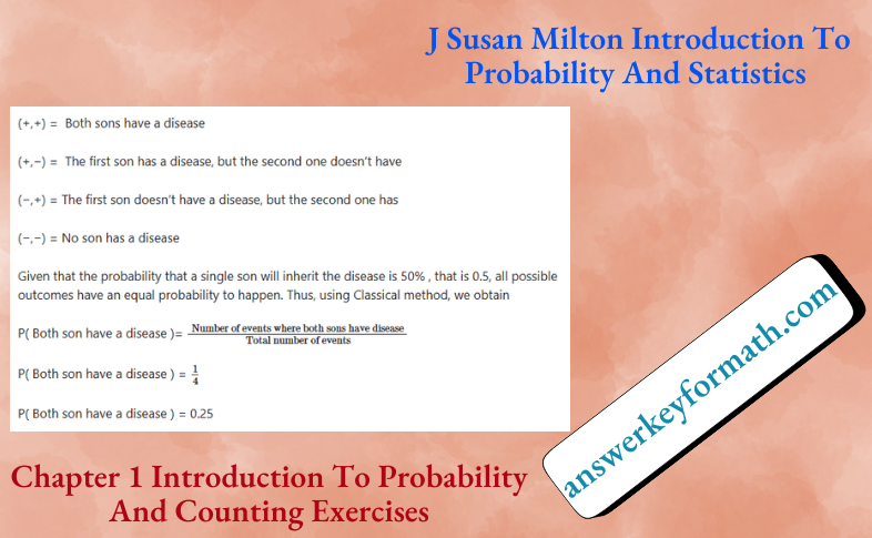
​The probability that the carrier gives birth to two sons is 0.25 and the approach we used to find the probability is Classical Method.

J Susan Milton Introduction To Probability And Statistics Chapter 1 Page 14  Exercise 3  Problem 3

According to the question, The probability of having a fatal accident in the work place is assessed using the fatal accident frequency rate (FAFR).

This rate is defined by

FAFR = Number of fatalities per1000workers during a working lifetime.

We need to find the approach to probability of an individual having fatal accident while at work.

Also, Find the approximate probability that a coal miner will suffer a fatal injury. Coal mining industry and is taken into account when computing the industry-wide FAFR of 4.

We need to explain how the rate could be so low while at least some of the components used in its computation are high.

Given that  FAFR = Number of fatalities per1000workers during a working lifetime.

Hence we use the relative frequency approach to approximate the given probability

Given that FAFR for coal mining occupation is 12

We use the relative frequency approach, hence we conclude that the probability that a coal miner will suffer a fatal injury is.

⇒ \(\frac{12}{1000}\)

=  0.012

The overall industry FAFR is equal to 4 because for a large number of occupations, FAFR is very low because those occupations are not dangerous and risky for human life.

The probability approach we used is relative frequency approach. The probability that a coal miner will suffer a fatal injury is 0.012. Coal mining industry and is taken into account when computing the industry-wide FAFR of 4, that is very low because those occupations are not dangerous and risky for human life.

Solutions To Probability And Counting Exercises Chapter 1 Susan Milton Page 15  Exercise 4  Problem 4

Questions explains that in ballistics studies conducted during World War II, it was found that inground-to-ground firing, artillery shells tended to fall in an elliptical pattern such as given in the question.

The probability that a shell would fall in the inner ellipse is 0.50 ; the probability that it would fall in the outer ellipse is 0.95.

A firing is considered to be a success (s)if the shell falls within the inner ellipse; otherwise, it is failure (f).

We need to construct a tree to represent the firing of four shells in succession.

For each of the four shells, we have two possible outcomes  (given shell falls within inner ellipse) or f (given shell doesn’t fall within inner ellipse).

Hence the tree diagram that represent the firing of four shells in succession as follows

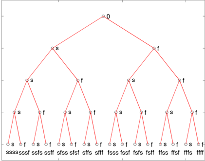
The tree diagram that represent the firing of four shells in succession as follows

J Susan Milton Introduction To Probability And Statistics Chapter 1 Page 15  Exercise 5 Problem 5

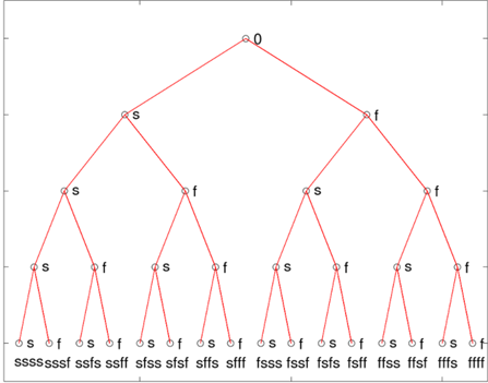
Questions explains that in ballistics studies conducted during World War II, it was found that inground-to ground firing, artillery shells tended to fall in an elliptical pattern such as given in the question.

The probability that a shell would fall in the inner ellipse is 0.50 ; the probability that it would fall in the outer ellipse is 0.95.

We need to list the sample points generated by the tree.

With the help of tree diagram from  Page 15  Exercise 4  Problem 4 , We conclude the sample space and sample points are:

S = {ssss,sssf,ssfs,ssff,sfss,sfsf,sfs,sfff,fsss,fssf,fsfs,fsff,ffss,ffsf,ffs,ffff}

The sample space and the sample points are: S={ssss,sssf,ssfs,ssff,sfss,sfsf,sff,sff,fsss,fssf,fsfs,fsff,ffss,ffsf,fff,ffff}

Probability and Statistics J. Susan Milton Chapter 1 solved step-by-step Page 15  Exercise 5  Problem 6

Questions explains that in ballistics studies conducted during World War II, it was found that inground-to ground firing, artillery shells tended to fall in an elliptical pattern such as given in the question.

The probability that a shell would fall in the inner ellipse is 0.50 ; the probability that it would fall in the outer ellipse is 0.95.

Let Ai,i = 1,2,34 denote the event that the i−thfiring is successful. We need to list the sample points that constitute each of the events A₁ ,A₂,A₃,A₄ and check are these events mutually exclusive.

The sample points that constitute each of the events A₁,A₂,A₃,A₄ are

A₁= the first firing is successfulsssss,sssf, ssfs,ssff,sfss,sfsf,sffs,sfff

A₂ = The second firing is successful{ssss,sssf,ssfs,ssff,fsss,fssf,fsfs,fsff}

A₃ = The third firing is successful{ssss,sssf,sfss,sfsf,fSSS,fssf,ffss,ffSf}

A₄ = The fourth firing is successful{sssss, ssfs, sfss, sffs, fsss, fsfs, ffss, fffs }

A,A₂,A₃,A₄ are not mutually exclusive events because event{ssss} is in every four events.

The sample points that constitute each of the events A₁,A₂ ,A₃,A₄  are

A₁ = {ssss,sssf,ssfs,ssff,sfss,sfsf,sffs,sfff}

A₂ = {ssss,sssf,ssfs,ssff,fsss,fssf,fsf,fsff

A₃ = {ssss,sssf,sfss,sfsf,fsss,fssf,ffss,ffsf}

A₄ = {ssss,ssfs,sfss,sffs,fsss,fsfs,ffs,fffs}

A₁, A₂, A₃, A₄ are not mutually exclusive events because event {ssss}is in every four events.

J Susan Milton Introduction To Probability And Statistics Chapter 1 Page 15  Exercise 5  Problem 7

Questions explains that in ballistics studies conducted during World War II, it was found that inground-to ground firing, artillery shells tended to fall in an elliptical pattern such as given in the question.

The probability that a shell would fall in the inner ellipse is 0.50; the probability that it would fall in the outer ellipse is 0.95.

We need to list the sample points that constitute each of these events and describe the events verbally:
​
​A₁′

A₁∪A₂

A₁∩A₂

A₁∩A₂∩A₃∩A₄

​A₁∩A₂∩A₃∩A′₄

(A₁∪A₂∪A₃∪A₄)A₁∩A′₁

​The sample points from the definition of complement, union and intersection

A₁′= The first firing is not successful{fSSS,fSSf,fsfs,fsff,ffS,ffsf,fffs,fff}

A₁∪A₂ = The first or second firing is successful{ssss,sssf,ssfs,ssff,sfss,sfsf,sffs,sfff,fsss,fssf,fsfs,fsff}

A₁∩A₂  =  The first and second firing is successfulsssss,sssf,ssfs,ssff}

A₁∩A₂∩A₃∩A₄ = All four firing are successful {ssss}

A₁∩A₂∩A₃∩A′₄= The first three firings are successful and the last one is not {sssf}

(A₁∪A₂∪A₃∪A₄)′ = All firings are unsuccessful {fff}

A₁∩A₁′= The first firing is successful and the first firing is not successful =Φ

The sample points from the definition of complement, union and intersection

A₁′ = {fSSS,fssf,fsfS,fSff,fSS,ffsf,ffS,fff}

A₁∪A₂ = {ssss,sssf,ssfs,ssff,sfs,sfsf,sffs,sfff,fsss,fssf,fsfs,fsff}

A1∩A₂ = {ssss,sssf,ssfs,ssff}

A₁∩A₂∩A₃∩A₄ = {sSSS}

A1∩A₂∩A₃∩A₄ = {sssf}

(A₁∪A₂∪A₃∪A₄) = {ffff}

A₁∩A₁′ = Φ

J Susan Milton Introduction To Probability And Statistics Chapter 1 Page 15  Exercise 5  Problem 8

Questions explains that in ballistics studies conducted during World War II, it was found that inground-to ground firing, artillery shells tended to fall in an elliptical pattern such as given in the question.

The probability that a shell would fall in the inner ellipse is 0.50 ; the probability that it would fall in the outer ellipse is 0.95.

We need to find the probability of each of the events of part(d) by classical probability and why is it true.

The probability for a single shell to fall when the inner ellipse is 0.5, then he probability for a single shell to fall outside of the inner ellipse is also 0.5.From the classical method we have:

P(A) = \(\frac{\text { Number of ways } A \text { can occur }}{\text { Number of ways the experiment can proceed }}\)

Each sample point can occur in one and only one way. Also, there are 16 possible outcomes in total. So, the probability of each sample point is: 1

= \(\frac{1}{16}\)

= 0.0625

The probability of each sample point is: 0.0625

Online help for J. Susan Milton Probability Chapter 1 exercises Page 16  Exercise 6  Problem 9

We need to evaluate the expression  9!

We have expression as  9!

​9! = 9 × 8 × 7 × 6 × 5 × 4 × 3 × 2 × 1

​9!  = 362880
​
The value of the expression 9! is 362880.

J Susan Milton Introduction To Probability And Statistics Chapter 1 Page 16  Exercise 6   Problem 10

We need to evaluate the expression 6!

We have expression as 6!

​6! = 6 × 5 × 4 × 3 × 2 × 1

​6!  = 720

​The value of the expression 6! is 720.

Step-by-step guide to Probability and Counting exercises Chapter 1 Milton Page 16  Exercise 6  Problem 11

We need to evaluate the expression  ₇P₃

We have expression as ₇P₃

​ ₇P₃  = \(\frac{7 !}{(7-3) !}\)

​ ₇P₃  =  \(\frac{7 !}{4 !}\)

​ ₇P₃  = \(\frac{7 \times 6 \times 5 \times 4 \times 3 \times 2 \times 1}{4 \times 3 \times 2 \times 1}\)

Cancilation of (4,3,2,1)

= 7 × 6 × 5

= 210
​
The value of the expression  ₇P₃  is 210.

Page 16  Exercise 6  Problem 12

We have expression as  ₆p₂

₆p₂ = \(\frac{6 !}{(6-2) !}\)

₆p₂ = \(\frac{6 !}{4 !}\)

₆p₂ =  \(\frac{6 \times 5 \times 4 \times 3 \times 2 \times 1}{4 \times 3 \times 2 \times 1}\)

Cancilation of (4,3,2,1)

= 6 × 5

= 30

The value of the expression ₆p₂  is 30. 

J Susan Milton Introduction To Probability And Statistics Chapter 1 Page 16  Exercise 6  Problem 13

According to the question, in investigating the ideal Gas Law, experiment are to be run at four different pressures and three different temperatures.

We need to find the number of experimental conditions are to be studied.

The multiplication principle: Consider an experiment taking place in k stages.

Let ni denote the number of ways in which stage i can occur for  i = 1,2,3,……k.

Altogether the experiment can occur in ways.

\(\prod_{i=1}^k\) ni = n₁ × n₂  n_k

Since we have four different pressures and three different temperatures, according to the multiplication principle, we conclude that  4 × 3 = 12 experimental conditions will be studied.

12 experimental conditions are to be studied.

Exercise solutions for Chapter 1 Susan Milton Probability and Counting Page 16  Exercise 6  Problem 14

According to the question, in investigating the ideal Gas Law, experiment are to be run at four different pressures and three different temperatures.

We need to find number of experiments will be conducted on the given gas if each experiment condition is replicated five times.

The multiplication principle: Consider an experiment taking place in k stages.

Let  n_i denote the number of ways in which stage  i can occur for i = 1,2,3,……k.

Altogether the experiment can occur in

\(\prod_{i=1}^k\) n_i = n₁ × n₂  n_k

Since, each experimental condition is repeated five times, from the multiplication principle, we conclude that 5 × 12 = 60 experimental conditions will be conducted on a given gas.

60 experimental conditions will be conducted on a given gas.

J Susan Milton Introduction To Probability And Statistics Chapter 1 Page 16  Exercise 6  Problem 15

According to the question, in investigating the ideal Gas Law, experiment is to be run at four different pressures and three different temperatures.

We need to find number of experiments will be conducted to obtain five replications on each experimental condition for each of the six different gases.

The multiplication principle: Consider an experiment taking place in k
stages.

Let n_i denote the number of ways in which stage i can occur for i = 1,2,3,……k.

Altogether the experiment can occur in

\(\prod_{i=1}^k\) n_i = n₁ × n₂  n_k

Since, each of six gases, there will be 60 conducted experiments from the multiplication principle, we conclude that 6 × 60 = 360

360 experiments will be conducted to obtain five replications on each experimental condition for each of the six different gases.

Page 17  Exercise 7  Problem 16

Four artillery shells have been fired in succession, each firing is either considered as a success or a failure.

We need to use the multiplication rule to prove that the number of paths through the tree for this experiment is 16.

There are four artillery shells, k = 4

The experiment is either a success or failure for i = 1,2,3,4

Therefore n₁ ,n₂,n₃ and n₄ are equal to 2.

From the multiplication principle

\(\prod_{i=1}^4 n_i\) = 2.2.2.2.

= 16

Number of paths through the tree representing this experiment is 16.

Using the multiplication principle, the number of paths through the tree to represent the experiment which involved firing of four artillery shells is proven to be 16.

J Susan Milton Introduction To Probability And Statistics Chapter 1 Page 17  Exercise 8  Problem 17

The Apollo mission consists of five components and each component is marked as operable or inoperable but for the proper functioning of this mission all the states must be operable.

We need to indentify the number of states that are operable.

In this mission the number of components are five, k = 5.

The components are either operable or inoperable for i = 1,2,3,4,5

Hence n₁ ,n₂,n₃,n₄ and n₅ is equal to 2.

Therefore, from the multiplication principle;

\(\prod_{i=1}^5 n_i\) = 2.2.2.2.2

= 32

The number of states that are operable is 32.

For the Apollo mission that consists of five components that is marked as either operable or inoperable, the number of states that are operable is found to be 32.

Page 17  Exercise 8  Problem 18

The Apollo mission consists of five components and each component is marked as operable or inoperable but for the proper functioning of this mission all the states must be operable.

We need to indentify the number of states in which LEM is inoperable.

The Apollo mission has five components in which if LEM is inoperable then the remaining states are four, k = 4.

The components are either operable or inoperable for i = 1,2,3,4

Therefore n₁ ,n₂ ,n₃ and n₄ are equal to 2.

From the multiplication principle

\(\prod_{i=1}^4 n_i\) = 2.2.2.2

= 16

The number of states in which the LEM is inoperable is 16.

For the Apollo mission that consists of five stages, the number of states when LEM Is inoperable is 16.

J Susan Milton Introduction To Probability And Statistics Chapter 1 Page 17  Exercise 8   Problem 19

The Apollo mission consists of five components and each component is marked as operable or inoperable but for the mission to be partially successful the first three components must be operable.

Therefore we need to find the number of states which represents, partially successful mission.

The mission has five components in which if the first three components are operable then the mission is considered as partially successful.

So we keep the first three components fixed and the last two components is either operable or inoperable hence according to the multiplication principle;

n₄  = n₅ ⇒ 2

= 2⋅2

= 4

The number of states that represent a partially successful mission

For the Apollo mission to be partially successful the first three components must be operable hence the number of states that represents a partially successful mission is 4.

Page 17  Exercise 8  Problem 20

The Apollo mission consists of five components and each component is marked as operable (o) or inoperable (i) but for the success of this mission all the states must be operable.

We need to in dentify the number of states when the mission is fully successful.

The operable state is denoted as (o) and the inoperable state is denoted as (i) For a complete successful mission all the five components must be operable and therefore the numbers of states that represent fully successful mission is ooooo.

For the Apollo mission to be fully successful the all five components must be operable hence the number of states that represents a fully successful mission is ooooo.

J Susan Milton Introduction To Probability And Statistics Chapter 1 Page 17  Exercise 9   Problem 21

Binary code consists of on (1) and off (0) values.

When each pixel is quantized to gray level using a binary code, we need to find how many gray levels can be quantized using a four bit binary code.

Four level binary code is there in which each binary digit is considered as a stage hence κ = 4

In binary system we have (0)’s and (1)’s hence  n₁,n₂,n₃ and n₄ are equal to 2.

From the multiplication principle

\(\prod_{i=1}^4 n_i\) = 2.2.2.2

The number of gray levels that are quantized using four bit binary system is 16.

The number of gray levels that are quantized using four bit binary system is 16.

Page 17  Exercise 9  Problem 22

Binary code consists of on (1) and off (0) values.

We need to find the number of bits required to code a pixel that is quantized to 32  grey levels

The number of bits required is the number of stages which is equal to k.

Since there are two possibilities0and 1 we have, 2⋅2⋅2⋅…⋅n_k = 32

2^k =  32

k = 5 since (25 = 32)

Therefore the number of bits of binary code that is required to code a pixel that is quantized to 32 grey levels is 5.

The number of bits of binary code that is required to code a pixel that is quantized to 32 grey levels is 5.

J Susan Milton Introduction To Probability And Statistics Chapter 1 Page 17  Exercise 10  Problem 23

We know that _nC_r= \(\left(\begin{array}{l}n \\r\end{array}\right)\) = \(\frac{n !}{r !(n-r) !}\) , hence we have to prove  _nC_r = _nC_n-r

We know that    _nC_r  = \(\left(\begin{array}{l}n \\r \end{array}\right) \Rightarrow \frac{n !}{r !(n-r) !}\)

So , C_n-r = \(=\left(\begin{array}{l}n \\n-r\end{array}\right) \Rightarrow \frac{n !}{(n-r) !(n-(n-r)) !}\)

C_n-r  = \(\frac{n !}{r !(n-r) !} \Rightarrow{ }_n C_r\)

Hence  _nC_r = _nC_n-r

Since _nC_r=\(\left(\begin{array}{l}n \\r\end{array}\right) \Rightarrow \frac{n !}{r !(n-r) !}\) and also  C_n-r =\(\left(\begin{array}{l}n \\n-r\end{array}\right)\)  \(\Rightarrow \frac{n !}{(n-r) !(n-(n-r)) !}\) , we prove that _nC_r =  _nC_n-r.

Page 17  Exercise 11  Problem 24

Given five compilers, pair wise comparisons are done hence we need to find the combinations of these five compilers selected two at a time.

The number of compilers is five, n = 5

Two are compared, r = 2

Substituting in the equation  _nC_r = \(\left(\begin{array}{l}n \\r\end{array}\right)\) \(\Rightarrow \frac{n !}{r !(n-r) !}\)

₅C₂ = \(\left(\begin{array}{l}5 \\2\end{array}\right) \Rightarrow \frac{5 !}{2 !(5-2) !}\)

₅C₂  = \(\frac{5 \cdot 4 \cdot 3 \cdot 2 \cdot 1}{2 \cdot 1(3 \cdot 2 \cdot 1)}\)

₅C₂  = \(\frac{20}{2}\)

₅C₂  = 10

The number of pair wise comparisons made are 10.

Given five compilers, the number of pair wise comparisons made are 10.

J Susan Milton Introduction To Probability And Statistics Chapter 1 Page 17  Exercise 12  Problem 25

We need to use the formula _nC_r = \(\frac{n !}{r !(n-r) !}\)

Where

n = 103 Is the pool of qualified applicants

r = 22 Is number of applications to select.

We need to find _nC_r  = \(\frac{n !}{r !(n-r) !}\)

Substituting values

_nC_r = \(\frac{n !}{r !(n-r) !}\)

Substituting values

_nC_r  ​⇒  \(\frac{103 !}{22 !(81) !}\)

_nC_r  ⇒ 1.51978828 × 1022

The number of ways 22 applications can be selected from a pool of 103 applications is 1.51978828 × 1022.

Page 17  Exercise 12  Problem 26

We need to use the formula = \(\frac{n !}{r !(n-r) !}\)

Considering that you are one of the applicants, we need to find the number of pools you will be included it.

Thus, of the 22 people, you are one of them and the other 21 people will be chosen from a pool of 102

Where

n = 102 is the pool of qualified applicants

r = 21 Is number of applications to select.

Substituting values

_nC_r  = \(\frac{n !}{r !(n-r) !}\)

_nC_r   ⇒ \(\frac{102 !}{21 !(81) !}\)

_nC_r   ​⇒ 3.25 × 10 ²¹

The number of sub-groups you will be included in is  3.25 × 10 ²¹.

J Susan Milton Introduction To Probability And Statistics Chapter 1 Page 17  Exercise 12  Problem 27

We need to find the probability of being selected considering all candidates are equal.

The number of times you will be in the pool of selected applicant is  3.25 × 10 ²².

The total number of ways pools can be formed is 1.52 × 10 ²²

We need to find the probability of getting selected.

Find the probability of being selected

P(A) = \(\frac{A}{B}\)

​⇒  \(\frac{3.25 \times 10^{21}}{1.52 \times 10^{22}}\)

​⇒ 0.21

The probability of getting selected from a pool of 103 applicants is 0.21.

J Susan Milton Introduction To Probability And Statistics Chapter 1 Page 18  Exercise 13  Problem 28

There are 128 – bit messages.

Each bit can be either correct or incorrect.

Hence, the total number of possible messages are 2 ²¹⁸

We need to find the number of cases where only two of these bits are wrong and the rest are correct.

For this we look at number of ways two bits can be selected of theone-twenty-eight.

Using that, we shall find the probability.

Find the number of events satisfying our condition

_nC_r = \(\frac{n !}{r !(n-r) !}\)

128 C₂ = \(\frac{128 !}{2 !(128-2) !}\)

Find the probability

The parobability of two of the bits being wrong

⇒ \(\frac{2-b i t s}{\text { Total }}\)

⇒ \(\frac{\frac{128 !}{2 !(128-2) !}}{2^{128}}\)

⇒ 2.39 10^{– 35}

⇒ \(\frac{127 \times 64}{2^{128}}\)

The probability of only two of the bits being wrong is 2.39 × 10^{– 35}

J Susan Milton Introduction To Probability And Statistics Chapter 1 Page 18  Exercise 13  Problem 29

There are \(\frac{n !}{n_{1} ! \times n_{2} ! \ldots n_{k} !}\) experiments with 4 different temperatures, each three times.

So, comparing with

n = n₁ + n₂ +…+ n_k

12  = 3 + 3 + 3 + 3

We need to find the number of ways the experiment can be conducted.\(\frac{n !}{n_{1} ! \times n_{2} ! \ldots n_{k} !}\)

Substituting into  \(\frac{n !}{n_{1} ! \times n_{2} ! \ldots n_{k} !}\)

⇒ \(\frac{12 !}{3 ! \times 3 ! \times 3 ! \times 3 !}\)

⇒ 369600

The number of ways the experiment can be conducted is 369600.

J Susan Milton Introduction To Probability And Statistics Chapter 1 Page 18  Exercise 13  Problem 30

We need to prove that \(\left(\begin{array}{c}
n \\
n_1
\end{array}\right)\left(\begin{array}{c}
n-n_1 \\
n_2
\end{array}\right) \ldots\left(\begin{array}{c}
n-n_1-n_2 \ldots n_{k-1} \\
n_k
\end{array}\right)\) = \(\frac{n !}{n_{1} ! \times n_{2} ! \ldots n_{k} !}\)

⇒ \(\frac{n !}{n_{1} !\left(n-n_1\right) !} \times \frac{\left(n-n_1\right) !}{n_{2} !\left(n-n_1-n_2\right) !} \cdots \cdot \frac{\left(n-n_1-n_2 \ldots n_{k-1}\right) !}{n_{k} !\left(n-n_1-n_2 \ldots n_k\right) !}\)

Every denominator of the numerator is cancelled out by the denominator of the previous term’s part leaving us with

⇒ \(\frac{n !}{n_{1} ! \times n_{2} ! \ldots n_{k} !(n-n) !}\)

Which is the RHS

We thus proved that \(\left(\begin{array}{c}n \\n_1\end{array}\right)\left(\begin{array}{c}n-n_1 \\n_2\end{array}\right) \ldots\left(\begin{array}{c}
n-n_1-n_2 \ldots n_{k-1} \\n_k\end{array}\right)\) =\( \frac{n !}{n_{1} ! \times n_{2} ! \ldots n_{k} !\left(n-n_1-n_2 \ldots n_k\right) !}\)

J Susan Milton Introduction To Probability And Statistics Chapter 1 Page 18  Exercise 14  Problem 31

We need to find n when

\(\left(\begin{array}{l}n \\2\end{array}\right)\) = 21 , \(\left(\begin{array}{l}n \\2\end{array}\right)\) = 105

We shall use the formula  \(\left(\begin{array}{l}
n \\
r
\end{array}\right)\) = \(\frac{n !}{r !(n-r) !}\)

For \(\left(\begin{array}{l}
n \\
2
\end{array}\right)\) = 21

Substituting in 

\(\left(\begin{array}{l}
n \\
r
\end{array}\right)=\frac{n !}{r !(n-r) !}\) 

= \(\frac{n !}{r !(n-r) !}\)

⇒ \(\frac{n !}{2 !(n-2) !}\) = 21

⇒ n(n – 1) = 21 (2)

⇒ n(n – 1) = 42

Thus we Know n = 7

For \(\left(\begin{array}{l}n \\2\end{array}\right)\) = 105

Substituting in 

⇒  \(\frac{n !}{r !(n-r) !}\)

⇒ \(\frac{n !}{2 !(n-2) !}\) 105

⇒ n(n – 1) = 105(2)

⇒  n(n – 1) = (15)(14)

Thus n = 15

For \(\left(\begin{array}{l}n \\2\end{array}\right)\)  = 21 , For \(\left(\begin{array}{l}n \\2\end{array}\right)\) = 105 , n = 15.

J Susan Milton Introduction To Probability And Statistics Chapter 1 Page 19  Exercise 15  Problem 32

There are 25 packages.

10 packages need to be chosen.

The number of ways this can be done is

⇒  \(\left(\begin{array}{l}25 \\10\end{array}\right)\).

Then we need to find ways to select 3 games  if  5 games packages exist within the given packages.

The number of ways this can be done is

⇒ \(\left(\begin{array}{l}20 \\7\end{array}\right)\) \(\left(\begin{array}{l}5 \\3\end{array}\right)\)

Finding \(\left(\begin{array}{l}20 \\7\end{array}\right)\) , \(\left(\begin{array}{l}5 \\3\end{array}\right)\)

⇒  \(\frac{20 !}{7 !(13) !} \times \frac{5 !}{3 !(2) !}\)

 = 775200

The number of ways 10 packages can be chosen is 3.27 × 10⁶. The number of ways three of these can be games is 775200.

J Susan Milton Introduction To Probability And Statistics Chapter 1 Page 19  Exercise 16  Problem 33

There are four women and six men.

We need to find the total number of ways three employees can be chosen at random.

Then we need to find the ways no women is chosen.

The ration of the two gives us the probability.

Total number of ways three employees can be chosen is

⇒ 240

Number of ways no women is chosen is the number of ways three men are chosen which is

⇒ 20

Probability that no women is chosen is

⇒ \(\frac{20}{240}\)

Which is \(\frac{1}{12}\).

Probability that no women is chosen is \(\frac{1}{12}\) As the probability is very low, the occurrence of such an event is suspicious as there is a god chance that at least one woman would be chosen if randomly chosen.

J Susan Milton Introduction To Probability And Statistics Chapter 1 Page 19  Exercise 17  Problem 34

We need to use five alphabets and one digit to make the password.

Any of the twenty six alphabets and ten digits can be used.

We need to find the total number of all possible passwords.

Repeating the alphabets is allowed.

The total number of passwords that can exist are
​
​(26)(26)(26)(26)(26)(10)

=118813760

​The total number of possible passwords are 118813760.

Page 19  Exercise 17  Problem 35

We need to use five alphabets and one digit to make the password.

Any of the twenty six alphabets and ten digits can be used.

We need to find the ways three As and two Bs can be used with an even digit.

There are 5 even digits.

Repeating the alphabets is allowed.

The total number of ways three As and two Bs can be used with an even digit

⇒  \(\left(\begin{array}{1}5 \\3\end{array}\right)\) 5

⇒ \(\frac{5 !}{3 ! 2 !}\) × 5 = 50

The total number of ways three As and two Bs can be used with an even digit is 50.

Page 19  Exercise 17  Problem 36

We need to find the ways three As and two Bs can be used with an even digit.

There are 5 even digits.

The total number of ways three As and two Bs can be used with an even digit is 50.

The probability of guessing the correct password of the fifty possibilities is \(\frac{1}{50}\).

J Susan Milton Introduction To Probability And Statistics Chapter 1 Page 19  Exercise  18  Problem 37

Given: An electrical control panel has three toggle switcheslabeled I, II, and III each of which can be either on (O)or off (F).

To find – Construct a tree to represent the possible configurations for these three switches.

For each switch we have two options on (O)and off (F).

Thus the three diagram is given with

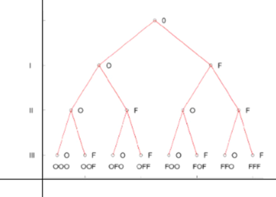
Hence, a tree to represent the possible configurations for these three switches is as follow:

J Susan Milton Introduction To Probability And Statistics Chapter 1 Page 19  Exercise  18  Problem 38

Given –  An electrical control panel has three toggle switches labeled I, II, and III each of which can be either on (O) or off(F).

To find –  List the elements of the sample space generated by the tree.

From the tree diagram we see that the sample space and sample points are S  {OOO,OOF,OFO,OFF,FOO,FOF,FFO,FFF}

Hence, from the elements of the sample space generated by the tree are S = {OOO,OOF,OFO,OFF,FOO,FOF,FFO,FFF}

J Susan Milton Introduction To Probability And Statistics Chapter 1 Page 19  Exercise  19  Problem 39

Given : An electrical control panel has three toggle switches labeled I, II, and III each of which can be either on (O) or off (F).

To find – What is the name given to an event such as D?

Event such as event D = 0 is called aa impossible event.

Hence, from the above explanation Event such as event D = 0 is called a impossible event.

Page 19  Exercise  19  Problem 40

Given:  Two items are randomly selected one at a time from an assembly line and classed as to whether they are of superior quality(+), average quality (0), or inferior quality (−)

To find – Construct a tree for this two-stage experiment.

For each of the two items we have tree oscillates. superior quality (+) average quality (0) or inferior quality (-) .

Thus the tree diagram a given with:

Hence, tree for this two-stage experiment is as follow

J Susan Milton Introduction To Probability And Statistics Chapter 1 Page 19  Exercise  19  Problem 41

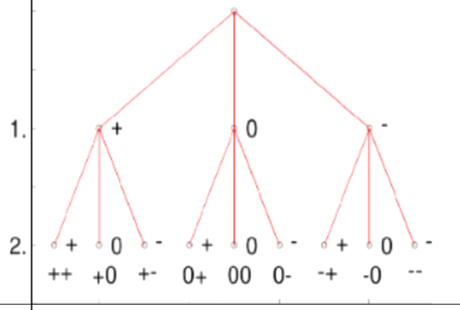
Given: Two items are randomly selected one at a time from an assembly line and classed as to whether they are of superior quality (+), average quality (0), or inferior quality (-)

To find – List the elements of the sample space generated by the tree.

From the tree diagram, we concluded that to sample space and sample points are S = {++,+0,+−,0+,00,0−,−+,−0,−−}

Hence, the elements of the sample space generated by the tree is as follow S = {++,+0,+−,0+,00,0−,−+,−0,−−}

Page 19  Exercise 19  Problem 42

Given: Two items are randomly selected one at a time from an assembly line and classed as to whether they are of superior quality (+), average quality (0), or inferior quality(−)

To find – List the sample points that constitute the events

A: The first item selected is of inferior quality

B: The quality of each of the items is the same

C: The quality of the first item exceeds that of the second

Using Page 19  Exercise 19   Problem 40   and Page 19  Exercise 19   Problem 41  we have

A = The first item selected is of inferior equal = {−+,−0,−−}

B = The quality of each of the items is the same = {++,00,−}

C = The quality of the First term exceeds that of the second = {+0,+−,0−}

Hence, the sample points that constitute the event are as follow:

A: The first item selected is of inferior quality ={−+,−0,−}

B: The quality of each of the items is the same={++,00,−−}

C: The quality of the first item exceeds that of the second ={+0,+−,0−}

J Susan Milton Introduction To Probability And Statistics Chapter 1 Page 20  Exercise  20   Problem 43

Given: An experiment consists of selecting a digit from among the digits 0 to 9 in such a way that each digit has the same chance of being selected as any other.

We name the digit selected A.

These lines of code are then executed.

IF A < 2 THEN B = 12;  ELSE B = 17

IFB = 12 THEN C = A − 1;  ELSE C = 0

To find – Construct a tree to illustrate the ways in which values can be assigned to the variables A, B, and C

From above given coordinate we have drawn a diagram :

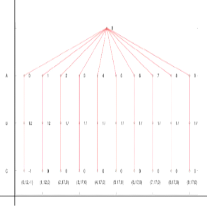
Hence:  A tree to illustrate the ways in which values can be assigned to the variables A, B, and C

J Susan Milton Introduction To Probability And Statistics Chapter 1 Page 20  Exercise 20  Problem 44

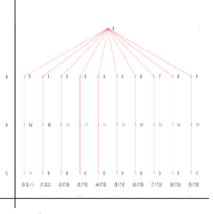
Given: An experiment consists of selecting a digit from among the digits 0 to 9 in such a way that each digit has the same chance of being selected as any other.

We name the digit selected A.

These lines of code are then executed.

IF A <2 THEN B = 12;  ELSE B = 17

IF B = 12 THEN C = A−1​; ELSEC = 0

To find –  Find the sample space generated by the tree.

From the tree diagraram, we see that the sample space and sample points are

S−{(0,12,−1),(1,12,0),(2,17,0),(3,17,0),(4,17,0),(5,17,0),(6,17,0),(7,17,0),(3,17,0),(9,17,0)\}

Hence, from the above explanation the sample space generated by the tree is as follow S−{(0,12,−1),(1,12,0),(2,17,0),(3,17,0),(4,17,0),(5,17,0),(6,17,0),(7,17,0),(3,17,0),(Officials at Nuclear Regulatory commission estimated the probability of such an accident occurring in the United States before the year to be by using Classical Method.9,17,0)\}

J Susan Milton Introduction To Probability And Statistics Chapter 1 Page 20  Exercise  20  Problem 45

Given: An experiment consists of selecting a digit from among the digits 0 to 9 in such a way that each digit has the same chance of being selected as any other. We name the digit selected A.

These lines of code are then executed.

IF A < 2 THEN B = 12;  ELSE B =  17

IF B = 12 THEN C = A-1; ELSE C = 0

To find –Find the probability that A is an even number.

The probability that A is an even number is the probability that A will be 0,2,4,6 or 8. so, there are five possibilities for A to be an even number and five to be an odd number.

Thus the probability that A is are even number is

5.\(\frac{1}{10}\) = \(\frac{1}{2}\)

Hence, from the above explanation the probability that A is an even number is 5.\(\frac{1}{10}\) = \(\frac{1}{2}\)

Introduction to Probability and Statistics Principles and Applications Chapter 2 Some Probability laws

Introduction To Probability And Statistics Chapter 2 Exercises Solutions Page 34  Exercise 1  Problem 1

The blood type distribution to be

A:  41%

B:  9%

AB:  4%

O:  46%

AB:  4%

O:  46%

We have to calculate the probability that the blood of a randomly selected individual will contain the antigen, it will contain the B antigen and it will contain neither the A nor the B antigen.

We have four possibilities for blood type and the probability of each of them is

​
Similarly, the blood of a randomly selected individual will contain the B antigen if his blood type is B or AB

Read and Learn More J Susan Milton Introduction To Probability And Statistics Solutions

Using the third axiom of probability we conclude

P(blood will contain the B antigen ) = P{B,AB}

P(blood will contain the B antigen ) = P(B) + P(AB)

P(blood will contain the B antigen ) = 0.09 + 0.04

P(blood will contain the B antigen ) = 0.13

In the same way, we conclude that the blood of a randomly selected individual will contain neither A nor the B antigen if and only if that person has blood type O Thus, P (blood will contain neither A nor the B antigen ) = P{O} = >0.46

The probability that the blood of a randomly selected individual will contain the A antigen is 0.45, it will contain the B antigen is 0.13 and it will contain neither the A nor the B antigen is 0.46

J. Susan Milton Probability Laws Chapter 2 Answers Page 34   Exercise 2   Problem 2

The engine component of a spacecraft consists of two engines in parallel.

The main engine is 95% reliable.

The backup is 80% reliable.

The engine component as a whole is 99% reliable.

We have to calculate the probability of both engines will be reliable.

We have to find a Venn diagram to find the probability that the main engine will fail but the backup will be operable.

And the probability that the backup engine will fail but the main engine will be operable.

We have to find the probability that the engine component will fail.

First, we define events A₁ and A₂ as

A₁ = The main engine will be operable

A₂ = The backup engine will be operable

From the text of exercise, we have

P (the main engine is operable) = P(A₁) = 0.95∣

P( the backup engine is operable ) = P(A₂) = 0.8

P( engine component is operable ) = P (at least one engine is operable) = P(A₁ ∪ A₂) = 0.99

Using the general addition rule

We can calculate the probability that both engines will be operable.

Thus, P (both engines will be operable) = P(A₁ ∩ A₂)

= P(A₁) + P(A₂) − P(A₁ ∪ A₂)

= 0.95 + 0.8 − 0.99

From the Venn diagram we conclude

P (the main engine is not operable and the backup is operable) = P(A₁ ∩ A₂)

P (the main engine is not operable and the backup is operable) ​= P(A₂) − P(A₁ ∩ A₂)

P (the main engine is not operable and the backup is operable) = 0.8 − 0.76

P (the main engine is not operable and the backup is operable) = 0.04

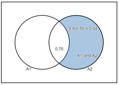
In the same way, we find the probability that the main engine will be operable and the backup engine will not be operable.

Hence, P (the main engine is operable and the backup engine is not operable)

​=  P(A₁) − P(A₁ ∩ A₂)

=  0.95−0.76

=  0.19
​

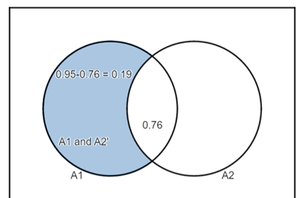
Since events A₁∩A₂, A′₁∩A₂, A₁∩A₂′are mutually exclusive, we can use the third axiom of probability.

Using that and the component rule we conclude
​
​P (Engine component will fail) = P (Both engines will fail)

​P (Engine component will fail) ⇒  ​P(A₁∩A₂′) = 1 − P(A′₁ ∩ A₂) − P(A₁ ∩ A₂′) − P(A₁ ∩ A₂)

​P (Engine component will fail) =  1 − 0.19 − 0.04 − 0.76

​P (Engine component will fail) =  0.01

​

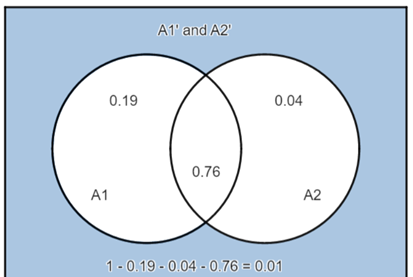
​The probability of both engines will be reliable is 0.76.

The probability that the main engine will fail but the backup will be operable from the Venn diagram is 0.04 . And the probability that the backup engine will fail but the main engine will be operable is 0.19.The probability that the engine component will fail is 0.01.

Solutions To Probability Laws Exercises Chapter 2 Susan Milton Page 35  Exercise 3  Problem 3

The axioms of probability are:

1. Let S donate a sample space for an experiment.

Then, P(S) = 1 ………….. (1)

2. For every event A, we have

P(A) ≥ 0 ………… (2)

3. Let A₁,A₂,A₃ ,……. be a finite or an infinite sequence of mutually exclusive events.

Then P(A₁ ∪ A₂ ∪ A ∪ …) = P(A₁) + P(A₂) + P(A₃) +  …………….. (3)

Let A be an arbitrary event.

Since from the definition of complement we have A∩A = θ,

We conclude that A and A ‘are mutually exclusive events.

So we can use axiom 3 for these two events.

Also since A ∪ A′ = S, we obtain
​
​1 =  P(S)

=  P(A ∪ A)

=  P(A) + P(A)
​
Thus
​
​1 =  P(A) + P(A)

⇒  P(A′) = 1 − P(A)

​So theorem is derived in the step section.

Chapter 2 Probability Laws Examples And Answers Susan Milton Page 35  Exercise 4   Problem 4

The axioms of probability are:

1.  Let S donate a sample space for an experiment.

Then, P(S) = 1 ……….. (1)

2. For every event A, we have

P(A) ≥ 0…………(2)

3. Let A₁,A₂,A₃ ,……. be a finite or an infinite sequence of mutually exclusive events.

Then P(A₁∪A₂∪A₃∪….) = P(A₁) + P(A₂) + P(A₃) +  ………… (3)

Let A be an arbitrary event.

Since A⊆S  We conclude

​​P(A) ≤ P(S) = 1

⇒ P(A) ≤ 1

​So theorem is derived in the step section.

Probability And Statistics J. Susan Milton Chapter 2 Solved Step-By-Step Page 35  Exercise 5  Problem 5

The axioms of probability are:

1. Let S donate a sample space for an experiment.

Then, P(S) = 1  …………..(1)

2. For every event A

We have P(A) ≥ 0 ….………… (2)

3. Let A₁, A₂, A3,… be a finite or an infinite sequence of mutually exclusive events.

Then P(A₁∪A₂∪A₃∪….)=P(A₁) + P(A₂) + P(A₃) + …..…….. (3)

Let A₁ and A₂  be arbitrary events.

Since A₁ = A₁ ∩ S

We obtain A₁ = A₁ ∩ S

= A₁ ∩ (A₂ ∪ A′₂)

=(A₁ ∩ A₂) ∪ (A₁ ∩ A′₂)

​Also, since A₂ ∩ A₂ = θ, we conclude

(A₁ ∩ A₂) ∩ (A1 ∩ A′₂) = θ

So, (A1 ∩ A₂) and (A1 ∩ A′₂)are mutually exclusive events and we can apply axiom 3 on these two events.

Similarly, since A₂ = A₂ ∩ S, we have

​A₂ = A₂ ∩ S = A₂ ∩ (A₁∪A₁′)

= (A₂ ∩ A₁) ∪ (A₂ ∩ A₁′)
​
Also, since A₁ ∩ A₁′z = θ

We conclude (A₂ ∩ A₁) ∩ (A₂ ∩ A₁′) =  θ

So A₂ ∩ A₁ are mutually exclusive events and we can apply axiom 3 on these two events.

Finally, for A₁ ∪ A₂, using the Venn diagram, we can conclude

A₁ ∪A₂ = (A₁ ∩ A₂) ∪ (A₁ ∩ A′₂)∪(A′₁ ∩ A₂)

Moreover, events A₁ ∩ A₂, A₁∩ A′₂, and A′₁ ∩ A₂  are mutually exclusive so we can apply axiom 3 on these three events.

From the above we have
​
​P(A₁)  =  P((A₁ ∩ A₂) ∩ (A₁ ∩ A₂′))

=   P(A₁ ∩ A₂) + P(A₁ ∩ A′₂)

P(A₂)  =  P ((A₂ ∩ A1) ∩ (A₂ ∩ A1))

=  P(A₂ ∩ A₁) + P(A₂ ∩ A′₁)

P(A₁ ∪ A₂)  =  P((A₁ ∩ A₂) ∪ (A₁ ∩ A′₂) ∪ (A₁ ∩ A₂))

=  P(A₁ ∩ A₂) + P(A₁ ∩ A′₂) + P(A′₁ ∩ A₂)
​
Finally we obtain
​
​P(A₁) + P(A₂) − P(A₁∩A₂)

​P(A₁) + P(A₂) − P(A₁∩A₂) = P(A₁ ∩ A₂) + P(A₁ ∩ A′₂) + P(A₁ ∩ A₂) + P(A′₁ ∩ A₂) − P(A₁ ∩ A₂)

​P(A₁) + P(A₂) − P(A₁∩A₂) = P(A₁ ∩ A₂) + P(A₁ ∩ A′₂) + P(A₁ ∩ A₂)

​P(A₁) + P(A₂) − P(A₁∩A₂) = P(A₁ ∪ A₂)

​The additional rule theorem is derived in the step section.

Online Help for J. Susan Milton Probability Chapter 2 Exercises Page 35  Exercise 6  Problem 6

When an individual is exposed to radiation, death may ensue.

Factors affecting the outcome are the size of the dose, the length and intensity of the exposure, and the biological makeup of the individual.

The term LD₅₀  is used to donate the dose that is usually lethal for 50% of the individuals exposed to it.

In a nuclear accident, 30%workers are exposed to the LD₅₀  and die.

40% of the workers die.

68% are exposed to the LD₅₀  or die.

We have to calculate the probability that a randomly selected worker will die given that he is exposed to the lethal dose of radiation.

First, we define events A and B as

A =  Randomly selected worker is exposed to the LD₅₀

B =  Randomly selected worker will die

From  we have P (A worker is exposed to the LD₅₀ and die)

=  P(A∩B) ⇒ 0.3

P( A worker will die ) = P(B) = 0.4

P(A worker is exposed to the LD₅₀ or die) = P(A∪B) ⇒ 0.68

P (A worker is exposed to the LD₅₀₎ = 0.58

P (A worker is exposed to the LD₅₀ but doesn’t die ) = 0.28P (A worker is not exposed to the LD₅₀  but dies ) = 0.1

We want to calculate P(B:A).

From the definition of conditional probability we conclude

​P(B:A) = \(\frac{P(A \cap B)}{P(A)}\)

​P(B:A)  =  \(\frac{0.3}{0.58}\)

​P(B:A)  =  0.5172

​The probability that a randomly selected worker will die given that he is exposed to the lethal dose of radiation is 0.5172.

Step-By-Step Guide To Probability Laws Exercises Chapter 2 Milton Page 35  Exercise 6  Problem 7

When an individual is exposed to radiation, death may ensue.

Factors affecting the outcome are the size of the dose, the length and intensity of the exposure, and the biological makeup of the individual.

The term LD₅₀ is used to donate the dose that is usually lethal for 50% of the individuals exposed to it.

In a nuclear accident, 30% workers are exposed to the LD₅₀ and die.

40%of the workers die.

68% are exposed to the LD₅₀ or die.

We have to calculate the probability that a randomly selected worker will not die given that he is exposed to the lethal dose of radiation

First, we define events A and B as

A =  Randomly selected worker is exposed to the LD₅₀

B = Randomly selected worker will die

From we have Page 35  Exercise 13  Problem 6

P(A worker is exposed to the LD ₅₀ and die ) = P(A ∩ B) ⇒ 0.3

P (A worker will die ) = P(B) ⇒ 0.4

P(A  worker is exposed to the LD₅₀ or die ) ⇒ P(A ∪ B) ⇒ 0.68

P(A  worker is exposed to the LD₅₀ ) = 0.58

P (A worker is not exposed to the LD₅₀ but dies ) = 0.1

We want to calculate P(B’:A)

From the definition of conditional probability we conclude

​P(B′: A) = \(\frac{P(A \cap B)}{P(A)}\)

​P(B′: A)  =  \(\frac{0.28}{0.58}\)

​P(B′: A)  = 0.4828

​We could also calculate that the probability in Page 35  Exercise 13 Problem 7 using the complement rule. 

Thus

​P(B′:A) ​= 1 − P(B’:A)

​P(B′: A)  = 1 − 0.5172

​P(B′: A)  =  0.4828

​The probability that a randomly selected worker will not die given that he is exposed to the lethal dose of radiation is 0.4828.

Exercise Solutions For Chapter 2 Susan Milton Probability Laws Page 35  Exercise 6  Problem 8

When an individual is exposed to radiation, death may ensue.

Factors affecting the outcome are the size of the dose, the length and intensity of the exposure, and the biological makeup of the individual.

The term LD₅₀ is used to donate the dose that is usually lethal for 50% of the individuals exposed to it.

In a nuclear accident, 30% workers are exposed to the LD₅₀ and die.

40% of the workers die.

68%are exposed to the LD₅₀ or die.

We have to find the theorem that allows to find the answer of Page 35  Exercise 13 Problem 7 with the knowledge of answer of  Page 35  Exercise 13  Problem 6.

First, we define events A and B as

A =  Randomly selected worker is exposed to the LD₅₀

B =  Randomly selected worker will die

From  we have Page 35  Exercise 13  Problem 6

P (A worker is exposed to the LD₅₀ and die)  = P(A ∩ B) ⇒ 0.3

P (A worker will die ) = P(B) = 0.4

P(A worker is exposed to the LD₅₀ or die ) = P(A ∪ B) ⇒ 0.68

P(A worker is exposed to the LD₅₀ ) = 0.58

P (A worker is exposed to the LD₅₀ but doesn’t die ) =  0.28

P (A worker is not exposed to the LD₅₀ but dies ) = 0.1

We could also calculate that the probability in Page 35  Exercise 13 Problem 7 using the complement rule.

Thus

​P(B′:A) = ​1 − P(B:A)

​P(B′:A)  =  1 − 0.5172

​P(B′:A)  =  0.4828
​
So with the help of the complement rule we can calculate the answer of Page 35  Exercise 13 Problem 7  from the knowledge of answer of Page 35  Exercise 13 Problem 6 .

Page 35  Exercise 6  Problem 9

When an individual is exposed to radiation, death may ensue.

Factors affecting the outcome are the size of the dose, the length and intensity of the exposure, and the biological makeup of the individual.

The term LD₅₀ is used to donate the dose that is usually lethal for50%of the individuals exposed to it.

In a nuclear accident, 30%workers are exposed to the LD₅₀ and die.

40% of the workers die.

68%are exposed to the LD₅₀ or die.

First, we define events A and B as

A =  Randomly selected worker is exposed to the LD₅₀

B =  Randomly selected worker will diel

From , we have Page 35  Exercise 13 Problem 6

P (A worker is exposed to the LD₅₀  and die)  = P(A ∩ B) ⇒ 0.3

P (A  worker will die) = P(B) = 0.4

P(A  worker is exposed to the LD₅₀  or die) = P(A ∪ B) ⇒ 0.68

P (A  worker is exposed to the LD₅₀ ) = 0.58

P(A worker is exposed to the LD₅₀ but doesn’t die) = 0.28

P(A worker is not exposed to the LD₅₀ but dies ) = 0.1

We want to calculate P(B:A′)

​Hece,P(B:A′)= \(\frac{\left.P(B \cap A)^{\prime}\right)}{P\left(A^{\prime}\right)}\)

P(B:A′) =  \(\frac{P(B \cap A)}{1-P(A)}\)

P(B:A′) ​=  \(\frac{0.1}{1-0.58}\)

The probability that a randomly selected worker will die given that he is not exposed to the lethal dose is 0.2381.

Page 35  Exercise 7  Problem 10

The engine component of a spacecraft consists of two engines in parallel.

The main engine is 95% reliable.

The backup is 80% reliable.

The engine component as a whole is 99% reliable.

We have to calculate the probability of both engines will be reliable.

We have to calculate the probability of both engines will be reliable.

We have to find a Venn diagram to find the probability that the main engine will fail but the backup will be operable.

And the probability that the backup engine will fail but the main engine will be operable.

We have to calculate the backup engine will function given that the main engine fails.

First, we define events A₁ and A₂ as

 A₁ = the main engine will be operable

A₂ = The backup engine will be operable

From the text of  exercise we have

P (The main engine is operable) = P(A₁) ⇒ 0.95

P( The backup engine is operable) = P(A₂) ⇒ 0.8

P( Engine component is operable ) = P( at least one engine is operable) = P(A₁ ∪ A₂)

= 0.99

P (Both engines will be operable) = P(A₁∩A₂) ⇒ 0.76

P (The main engine is not operable and the backup is operable) = P(A₁ ∩ A₂)  ⇒ 0.04

P (The main engine is operable and the backup engine is not operable) = P(A₁ ∩ A′₂)

= 0.19

P( Engine component will fail ) = P (both engines will fail) = P(A₁ ∩ A′₂)

= 0.01

We have to calculate P(A₂:A₁′)

From the definition of conditional probability we have

​P(A₂:A₁′)= \(\frac{P\left(A_2 \cap A_1^{\prime}\right)}{P\left(A_1^{\prime}\right)}\)

​P(A₂:A₁′) = \(\frac{P\left(A_2 \cap A_1^{\prime}\right)}{1-P\left(A_1\right)}\)

​P(A₂:A₁′) ​= \(\frac{0.04}{1-0.95}\)

​P(A₂:A₁′) = 0.8

The probability that, in an engine system such as that described, the backup engine will function given that the main engine fails 0.8

Page 35  Exercise 7   Problem 11

The engine component of a spacecraft consists of two engines in parallel.

The main engine is 95% reliable.

The backup is 80% reliable.

The engine component as a whole is 99% reliable.

We have to calculate the probability of both engines will be reliable.

We have to find a Venn diagram to find the probability that the main engine will fail.willfaiheWe wilfailbutthemai

First, we define events A₁ and A₂ as

A₁ = The main engine will be operable

A₂ = The backup engine will be operable

From the text of exercise, we have

P (The main engine is operable)

=  P(A1) = > 0.95

P (the backup engine is operable) = P(A₂ ) ⇒ 0.8

P( Engine component is operable )= P( At least one engine is operable )

= P(A₁∪A₂ ) = > 0.99

P (Both engines will be operable) = P(A₁∩A₂)

= 0.76

P (The main engine is not operable and the backup is operable) = P(A₁ ∩ A₂ ) ⇒ 0.04

P (The main engine is operable and the backup engine is not operable) = P(A₁ ∩ A′₂) ⇒ 0.19

P( Engine component will fail )= P( both engines will fail ) = P(A′₁ ∩ A₂′)

= 0.01

From

P( Backup functions) =  P(A₂) ⇒ 0.8

On the other side, from Page 35  Exercise 14  Problem 11 we have

P (backup function: main fails) = P(A₂:A′₁) ⇒ 0.8

So these two probabilities are equal.

This is not unusual because engines are in parallel. That is, they work independently of each other. Thus the probability that the backup engine will be operable does not depend in the working slate of the main engine.

Page 35  Exercise 8   Problem 12

In a study of waters near power plants and other industrial plants that release wastewater into the water system, it was found that 5% showed signs of chemical and thermal pollution 40% showed signs of chemical pollution.

35% Showed evidence of thermal pollution.

We have to calculate the probability that a stream that shows some thermal pollution will also show signs of chemical pollution.

And also the probability that a stream showing chemical pollution will not show signs of thermal pollution.

First, we define events A₁ and A₂ as

A₁= A stream shows signs of chemical pollution

A₂ = A  stream shows signs of thermal pollution

From the text of exercise, we have
​
​P(A) = 0.4

P(B) =  0.35

P(A∩B) = 0.05 = 0.76
​
We have to calculate the probability that a stream that shows thermal pollution will also show signs of chemical pollution, that is P(A⋮B).

Using the definition of conditional probability we obtain

P(A:B) = \(\frac{P(A \cap B)}{P(B)}\)

P(A:B) = \(\frac{0.05}{0.35}\)

P(A:B) = \(\frac{1}{7}\)

Now we will calculate the probability that a stream some chemical pollution will not show signs of thermal pollution, that is P(B:A).

Again using the definition of conditional probability we conclude

​P(B′:A)= \(\frac{P(A \cap B)}{P(B)}\)

​P(B′:A) = \(\frac{0.4}{0.05}\)

​P(B′:A) = \(\frac{7}{8}\)

The probability that a stream that shows some thermal pollution will also show signs of chemical pollution  \(\frac{7}{8}\). And also the probability that a stream showing chemical pollution will not show signs of thermal pollution  \(\frac{7}{8}\)

Page 36  Exercise 9   Problem 13

Given Data – A₁ and A₂ are independent events.

And P(A₁) = .5,  P(A₁) = .7

To be found – The value of P(A₁ ∩ A₂)

For Independent events A₁ and A₂

P(A₁∩A₂ ) = P(A₁)  ×  P(A₂)

Therefore = .5 × .7  (Substituting the values)

P(A₁∩A₂ )  = .35    (After simplification)

“For the given values of P(A₁) and P(A₂),the value of P(A₁ ∩ A₂ ) = .35.

Page 36  Exercise 10  Problem 14

Given Data –  P(A₁) = .6, P(A₂) = .4, P(A₁ ∪ A₂) = .8

To be found –  If A₁ and A₂ are independent events

We know

For two events A₁ and A₂

​P(A₁∪A₂) = P(A₁) + P(A₂) − P(A₁ ∩ A₂)

.8 =.6 + .4 − P(A₁ ∩ A₂) ​   (Substituting the values)

P(A₁ ∩ A₂) = .6 + .4 −.8     (After simplification)

P(A₁ ∩ A₂) =  .2                (After simplification)

We know for independent events A₁ and A₂

Now ⇒   P(A₁ ∩ A₂) = ​P(A₁) × P(A₂)

P(A₁ ∩ A₂) ≠ P(A₁) × P(A₂)

= .6 × .4 ​ (Substituting the values)

= 2.4      (After simplification)
​
Clearly, Therefore, A₁ and A₂ are not independent events.

For the given values of P(A₁) and P(A₂), A₁ and A₂ are not independent events.”

Page 36  Exercise 11  Problem 15

When an individual is exposed to radiation, death may ensue.

Factors affecting the outcome are the size of the dose, the length and intensity of the exposure, and the biological makeup of the individual.

The term LD₅₀  is used to donate the dose that is usually lethal for 50 % of the individuals exposed to it.

In a nuclear accident, 30 % workers are exposed to the LD₅₀ and die.

40%  Of the workers die.

68 %  Are exposed to the LD₅₀ or die.

First, we define events A and B as

A₁ = Randomly selected worker is exposed to the LD₅₀

A₂ = Randomly selected worker will die

From  Page 35  Exercise 6  Problem 9 , we have

P(A worker will die) = P(A₂) = 0.4

P(A worker will die: A  worker is exposed to lethaldose) = P(A₂:A₁) = 0.5172

Events, A₁ and A₂ are independent if and only if

P(A₁ ∩ A₂) = P(A₁)P(A₂)

If A₁ and A₂ are independent, then

P(A₂;A₁) = \(\frac{P\left(A_1 \cap A_2\right)}{P\left(A_1\right)}=\frac{P\left(A_1\right) P\left(A_2\right)}{P\left(A_1\right)}\) = P(A₂)

Since we have

P(A₂⋮A₁) = 0.5172 ≠ 0.4 = P(A₂)

We conclude that A₁ and A₂ are not independent.

The events A₁: A worker dies and A₂:The worker is exposed to a lethal dose of radiation are not independent.

Page 36  Exercise 12  Problem 16

The engine component of a spacecraft consists of two engines in parallel.

The main engine is reliable 95%.

The backup is 80 % reliable.

The engine component as a whole is 99 %reliable.

We have to find that the events

A1: The backup engine functions and 

A₂: The main engine fails are independent or not.

First, we define events A₁ and A₂ as

A₁ = The main engine will be operable

A₂ = The backup engine will be operable

From the text of exercise, we have

P(The backup engine is operable) = P(A₂) ⇒ 0.8

P(The main engineis fails: the backup engine functions)

= P(A₂⋮A₁) ⇒ 0.8

Events A₁  and A₂ are independent if and only if

P(A₁ ∩ A₂) = P(A₁)P(A₂)

From the definition of conditional probability, we have

P(A₁ ∩ A₂) = P(A₂⋮A₁)P(A₁)

⇒  P(A₂)P(A₁)

So Events A₁ and A₂ independent.

The events A1:The backup engine functions and A₂: The main engine fails are independent.

Page 36  Exercise 13  Problem 17

In a study of waters near power plants and other industrial plants that release wastewater into the water system, it was found that 5 % showed signs of chemical and thermal pollution 40 % showed signs of chemical pollution.

35 % Showed evidence of thermal pollution.

We have to test for independency of the events

A_{1 =} A stream shows signs of thermal pollution and 

A_{2 =} A stream shows signs of chemical pollution.

First, we define events as A₁ and A₂

P(A stream shows signs of thermal pollution) = P(A₁) = 0.35

P(A stream shows signs of chemical pollution) = P(A₂) = 0.4

P(A₂ ∩ A₁ ) = 0.05

Events A₁ and A₂ are independent if and only if

P(A₁ ∩ A₂) = P(A₁)P(A₂)

Since we have

​P(A₁) P(A₂) = 0.35 × 0.4 = 0.14 ≠ 0.05  = P(A₁ ∩ A₂)
​
We conclude that events A₁ and A₂ are not independent.

The events A₁: A stream shows signs of thermal pollution and A₂: A stream shows signs of chemical pollution are not independent.

Page 36  Exercise 14  Problem 18

Given Data – 

1) Probability of the event that the stream has high BOD is 0.35

2) Probability of the event that the stream has high Acidity is 0.1

3) Probability of the event that the stream has both high BOD and high Acidity is 0.04

We have to check if the events, the stream has high BOD and high Acidity are Independent or Not.

Let A be the event that the stream has high BOD.

And let $B$ be the event that the stream has high Acidity.

According to the question

​P(A) = 0.35

P(B) = 0.1

P(A ∩ B) = 0.04

Now

​P(A) × P(B) = 0.35 × 0.1

​P(A) × P(B)  =  0.035  (Substituting the values)

Therefore, A and B are not independent.

“For the given values of – probability of the event that the stream has high BOD  0.35 , probability of the event that the stream has high Acidity 0.1 , the stream has both high BOD and high Acidity 0.04, the events, the stream has high BOD and high Acidity are Not independent.

Page 36  Exercise 15  Problem 19

Given Data –

1.  Probability of the event that the individual inherited the negative Rh gene from father is 0.39

2. Probability of the event that the individual inherited the negative Rh gene from mother is 0.39

To be found – The probability that a randomly selected individual will have negative Rh blood

Let A be the event that the individual inherited the negative Rh gene from father.

And let B be the event that the individual inherited the negative Rh gene from mother.

According to the question

​P(A) = 0.39

P(B) = 0.39
​
Now, the possibility that a randomly selected individual will have negative Rh blood is possible when the individual will inherit negative Rh gene from both parents.

Therefore, the probability that a randomly selected individual will have negative Rh blood

=  P(A) × P(B)  ( A and B are independent events)

=  0.39 × 0.39  (Substituting the values)

=  0.1521  (After Multiplication)

​=  P(A∩B)  (Substituting the values)

“For the given values of – probability of the event that the individual inherited the negative Rh gene from father 0.39, probability of the event that the individual inherited the negative Rh gene from mother 0.39, the probability that a randomly selected individual will have negative Rh blood is 0.1521′′

Page 36 ​ Exercise 16   Problem 20

​An individual’s blood group (A,B,AB,O)is independent of the Rh classification.

We have to find the probability that a randomly selected individual will have AB negative blood.

First, we define events A₁ and A₂ as P(a randomly selected individual has AB blood type) = P(AB) ⇒ 0.04

P(a randomly selected individual has Rh​negative blood type) = P(Rh−) ⇒ 0.1521

We want to calculate the probability, that a randomly selected individual will have AB − blood type, that is P(AB∩Rh−).

Also from the text we conclude that AB and Rh− are independent events.

Thus P(AB∩Rh−) = P(AB)P(Rh−)

P(AB∩Rh−) =  .04 × 0.1521

P(AB∩Rh−) =  0.006084

The probability that a randomly selected individual will have AB negative blood is 0.006084.

Page 36  Exercise 17  Problem 21

Given Data – 

1. Probability of the event that the copper content will be high is 0.3

2. Probability of the event that the mint will be present is 0.23

3. Probability of the event that the mint will be present given copper content is high is 0.7

To be found – The probability that the copper content will be high and the mint will be present

Let A be the event that the copper content will be high.

And let B be the event that the mint will be present.

According to the question

​P(A) = 0.3

P(B) = 0.23

P(B/A) = 0.7
​
Now, the probability that the copper content will be high and the mint will be present
​
​= P(A∩B)   (Substitute the values) and (After multiplication)

= P(B/A) P(A)

=  0.7 × 0.3

=  0.21

For the given values of – probability of the event that the copper content will be high 0.3, probability of the event that the mint will be present   0.23 , probability of the event that the mint will be present given copper content is high 0.7, the probability that the copper content will be high and the mint will be present is0.21′′

Page 36  Exercise 17  Problem 22

Given Data – 

1. Probability of the event that the copper content will be high is 0.3

2. Probability of the event that the mint will be present is0.23

3. Probability of the event that the mint will be present given copper content is high is 0.7

To be found – The probability that the copper content will be high given that the mint i

Let A be the event that the copper content will be high.

And let B be the event that the mint will be present.

According to the question

​P(A) = 0.3

P(B) = 0.23

P(B/A) = 0.7
​
From  P(A ∩ B) = 0.21

Now, the probability that the copper content will be high given that the mint is present
​
​= P(A/B)

P(A/B) = \(\frac{P(A \cap B)}{P(B)}\)

​ P(A/B) = \(\frac{0.21}{0.23}\)  (Substituting the values)

P(A/B) =  0.91304 (After Multiplication)

“For the given values of – probability of the event that the copper content will be high0.3, probability of the event that the mint will be present 0.23, probability of the event that the mint will be present given copper content is high0.7, the probability that the copper content will be high given that mint is present is 0.91304”

Page 36  Exercise 17  Problem 23

Given Data –

1. Probability of the event that the copper content will be high is 0.3

2. Probability of the event that the mint will be present is 0.23

3. Probability of the event that the mint will be present given copper content is high is 0.7

To check if-The events the copper content will be high and the mint will be present are independent or not.

Let A be the event that the copper content will be high.

And let B be the event that the mint will be present.

According to the question

​P(A) ​= 0.3

P(B) = 0.23

P(B/A) =0.7

From  P(A∩B) = 0.21

Now P(A) × P(B)

P(A) × P(B) ​= 0.3 × 0.23

P(A) × P(B) = 0.069

(Substituting the values)  and  (After Multiplication)

Clearly P(A∩B) ≠ P(A) × P(B)

Therefore A and B are not independent.

“For the given values of – probability of the event that the copper content will be high 0.3, probability of the event that the mint will be present  0.23, probability of the event that the mint will be present given copper content is high 0.7, the events that the copper content will be high and the mint will be present are not independent.”

Page 37 Exercise 18  Problem 24

Given Data – 

1. Probability of the event that a randomly chosen person is asked the first question about the barn is 0.5

2. Probability of the event that a randomly chosen person claims to have seen the nonexistent barn was asked the first question about the barn is 0.17

3. Probability of the event that a randomly chosen person claims to have seen the nonexistent barn was not asked the first question about the barn is 0.03

To be found –  The non existent barn.

Let A₁ be the event that a randomly chosen person is asked the first question about the barn.

So A₁^c  will be the event that a randomly chosen person is not asked the first question about the barn.

And let A₂  be the event that a randomly chosen person claims to have seen the nonexistent barn.

Therefore, according to question

​P(A₁) = 0.5

P(A₂/A₁) = 0.17

P(A₂/A₁^c ) = 0.03
​
Since, A₁ and A₁^c are mutually exclusive. 

Therefore, A₂ ∩ A₁ and A₂ ∩ A₁ care also mutually exclusive.

Therefore ,P(A₂) = P(A₂ ∩ S)

As Union of a event and its complement forms the entire

Sample Space Therefore

​= P( A₂ ∩ (A₁ ∪ A₁^c  ))

= P((A₂ ∩ A₁) ∪ (A₂ ∩ A₁^c  ))

= P(A₂∩A₁) + P(A₂ ∩ A₁^c  )

= P(A₁)P(A₂/A₁) + P(A₁^c )(A/A₁^c  )

= 0.5 × 0.17 + (1−0.5) × 0.03   (Substituting the values)

= 0.5 × 0.17 + 0.5 × 0.03   (After Subtraction)

= 0.085 + 0.015   (After Multiplication)

= 0.1  (After Addition)

“For the given values of – Probability of the event that a randomly chosen person is asked the first question about the barn 0.5, Probability of the event that a randomly chosen person claims to have seen the nonexistent barn was asked the first question about the barn 0.17, Probability of the event that a randomly chosen person claims to have seen the nonexistent barn was not asked the first question about the barn 0.03, the probability of the event that a randomly chosen person claims to have seen the nonexistent barn is 0.1”

Page 37  Exercise 19  Problem 25

Given Data –

1. Probability of the event that the donor is paid is 0.67

2. Probability of the event that the patient has received a contracted serum hepatitis from paid donor is 0.0144

3.  Probability of the event that the patient has received a contracted serum hepatitis from unpaid donor is 0.0012

To be found the probability of the event that patient has received a contracted serum hepatitis

Let A₁ be the event that the donor was paid.

So A₁^c  will be the event that the donor was not paid.

And let A₂ is the event that patient has received a contracted serum hepatitis.

Therefore, according to question

P(A₁) = 0.67

P(A₂/A₁) = 0.0144

P(A₂/A₁^c ) = 0.0012
​
Since, A₁ and A₁^c care mutually exclusive.

Therefore, A₂ ∩ A₁ and A₂ ∩ A₁^c are also mutually exclusive.

Therefore P(A₂) = P(A₂∩ S)

As Union of a event and its complement forms the entire

Sample Space

Therefore

=  P (A₂ ∩ (A₁ ∪ A₁^c ))

​=  P ((A₂ ∩ A₁) ∪ (A₂ ∩ A₁^c  ))​

=  P(A₂ ∩ A₁) + P(A ∩ A₁^c )

=  P(A₁)P(A₂/A₁) + P(A₁^c )(A/A₁^c )

=  0.67 × 0.0144 + (1−0.67) × 0.0012   (Substituting the values)

= 0.67 × 0.0144 + 0.33 × 0.0012   (After Subtraction)

=  0.009648 + 0.000396   (After Multiplication)

=  0.010044     (After Addition)

“For the given values of – Probability of the event that the donor is paid 0.67 , Probability of the event that the patient has received a contracted serum hepatitis from paid donor 0.0144,Probability of the event that the patient has received a contracted serum hepatitis fromunpaid donor 0.0012, the probability of the event that patient has received a contracted serum hepatitis is 0.010044”

Page 37 Exercise 20  Problem 26

Given Data – Two events, one of which is impossible, and any other event

To prove that – The impossible event is always independent of any other event

Let the impossible event be A and any other event be B

Therefore

P(A) = 0 (Probability of impossible event is always Zero)

Also, an impossible event can never happen together with any other event.

Therefore, Impossible events are always mutually exclusive with other events.

Therefore, ​P(A∩B) = 0 (As A and B are mutually exclusive events)

Therefore Now

​P(A ∩ B)= 0 ​ (As A and B are mutually exclusive events)

P(A) × P(B) = 0 × P(B)    (Substituting the value of P(A))

=   0​              (After simplification)

Therefore, ​P(A∩B) = P(A) × P(B)​(Both Zero)

Therefore, A and B are not independent events.

“For the given events, one of which is impossible, and any other event, The events are independent.”

Page 37 Exercise 21  Problem 27

Given

A₁ = [A₁ ∩ A₂] ∪ [A₁ ∩ A′₂]

We have to show that if A₁ and A₂ are independent, then A₁ and A′₂ are also independent

Since A₁ and A₂  are independent, then  P[A₁ ∩ A₂] =  P[A₁]⋅P[A₂]

It is to be known that A₂ and A′₂ are mutually exclusive, then A₁ ∩ A₂ and A₁ ∩ A′₂ are also mutually exclusive.

Then P[A₁] = P[A₁ ∩ S]

= P[A₁ ∩ (A₂ ∪ A′₂)]

From the complement rule, we have A′₂

= 1 − P[A₂]

Hence, P[A₁ ∩ (A’₂)] = P[A₁]

P[A₁ ∩ A₂] = P[A₂]

⇒  P[A₁]P[A₂]

=  P[A₁] P[1 − A₂]

=  P[A₁]P[A′₂]

Therefore, A₁ and A′₂ are also independent.

Hence it is proved that A₁ and A′₂ are also independent.

Page 37  Exercise 22  Problem 28

According to the question, we need to use exercise 31 to show that if A₁ and A​′₂ are independent, then A′₁ and A′₂ are also independent.

If A₁ and A₂ are independent, from Page 37 Exercise 21  Problem 27, then we know that A₁ and A​′₂ are also independent

Thus, P (A₁ ∩ A​′₂) = P(A₁)P(A​′₂)……………………………… (1)

Since A′₁ and A′₂ are mutually exclusive, then A₁∩A′₂ and A′₁ ∩ A′₂ are also mutually exclusive so

P(A​′₂) = P(A′₂ ∩ S)…………(2)

= P(A′₂ ∩ (A₁ ∪ A′₁))

=P((A′₂ ∩ A₁) ∪ (A′₂ ∩ A′₁))

= P(A′₂ ∩ A₁) + P(A′₂ ∩ A′₁)

​We use complement rule ………………………(3)

From the above(1),(2),(3)equation, we get:
​
P(A′₂ ∩ A′₁) = P( A​′₂) − P(A₁ ∩ A​′₂)

= P(A′₂) − P(A₁)P(A′₂)

= P(A′₂)(1 − P(A₁))

= P(A′₂) P(A′₁)

So, A′₁ and A′₂ are independent.

With the help of  Exercise 31, Mutual exclusive and complement rule we have proved that A′₁ and A′₂ are also independent.

Page 37  Exercise 23  Problem 29

According to the question, it can be shown that the result of exercise 32 holds for any collection of n independent events.

That is, if A₁,A₂, ………………An are independent, then A′₁,A′₂,………………A′_n are also independent.

With the help of this result and data of example 2.3.4 we need to find the probability that at least one of the three computers will be operable at the time of the launch.

From example 2.3.4 we have

A₁  = The main system is operable

A₂ = The first backup is operable

A₃ = The second backup is operable.

Also, P(A₁) ⇒ P(A₂) ⇒ P(A₃) ⇒ 0.9

To calculate the probability that at least one system is operable, P(A₁ ∪ A₂ ∪ A₃), we use complement rule:

P(A₁ ∪ A₂ ∪ A₃)

= P  (At least one system is operable)

= 1 − P  (No system is operable)

= 1−P (A′₁ ∩ A′₂ ∩ A′₃)
​
Since, A₁ ,A₂,A₃  are independent, we say that A′₁,A′₂,A′₃ are also independent, Thus:

P(A′₁  ∩ A′₂ ∩ A′₃) = P(A′₁) ∩ P(A′₂) ∩ P(A′₃)

The probability that at least one system will be operable is:

​P(A₁ ∪ A₂ ∪ A₃) = 1−P(A′₁ ∩ A′₂ ∩ A′₃)

​P(A₁ ∪ A₂ ∪ A₃)  = 1−P(A′₁)(A′₂)(A′₃)

​P(A₁ ∪ A₂ ∪ A₃)  = 1−((1 − P(A₁)(1 − P(A₂)(1 − P(A₃))
​
​​P(A₁ ∪ A₂ ∪ A₃)  = 1 − ((1 − 0.9)(1 − 0.9)(1 − 0.9))

​P(A₁ ∪ A₂ ∪ A₃)  = 1 − (0.1 × 0.1 × 0.1)

​P(A₁ ∪ A₂ ∪ A₃)  = 1 − 0.001

​P(A₁ ∪ A₂ ∪ A₃)  = 0.999

​The probability that at least one system will be operable is 0.999

Page 37  Exercise 24  Problem 30

According to the question, let A₁  and A₂ be mutually exclusive events such that P(A₁)P(A₂ ) > 0.

We need to show that the events are not independent.

If A₁ and A₂ be mutually exclusive events such that  A₁ and A₂ be mutually exclusive events such that P(A₁ ∩ A₂ ) = P(Φ) = 0<P(A₁ )P(A₂ )

Hence, we see that  P(A₁∩ A₂ ) ≠ P(A₁ )P(A₂ ) ,events A₁ and A₂ are not independent.

Events A₁ and A₂ are not independent as P(A1 ∩A₂  )≠ P(A₁ )P(A₂).

Page 37 Exercise 25  Problem 31

According to the question, let A₁ and A₂ be independent events such that P(A₁)P(A₂ )>0.

We need to show that the events are not mutually exclusive.

If A₁ and A2 be independent events such that P(A₁∩A₂) = P(A₁) × P(A₂)

Given that  A₁ and A₂  be independent events such that  0 < P(A₁) P(A₂)

Now, we have  P(A₁ ∩ A₂) =  P(A₁) × P(A₂)>0

Hence, we see that P(A₁ ∩ A₂) > 0 A₁ and A₂ are can’t be mutually exclusive because to satisfy the mutually exclusive condition we need  P(A₁ ∩ A₂) = 0.

A₁ and A₁ are can’t be mutually exclusive because to satisfy the mutually exclusive condition we need  P(A₁∩A₂) = 0 but we have P(A₁∩A₂)>0.

Page 38   Exercise 26  Problem 32

We have to find the probability that who was typed as having type A blood actually had type B blood.

A = Inductee has type A blood

B =  Inductee has type B blood

AB =  Inductee has type AB blood

O =  Inductee has type O blood

TB =   Inductee is typed as type B blood

Also given that

P[A] = 0.41

P[TB/A​] = 0.88

P[B] = 0.09

P[TB/B​] = 0.04

P[AB] = 0.04

P[TB/AB​] = 0.10

P[O] = 0.46

P[TB/O​] = 0.04

We have to calculate P[B/TB​]

∴ P[B/TB​] = \(\frac{P[B \cap T B]}{P[T B]}\)

P[B∩TB] = P[TB/B​]⋅P[AB]

​=  (0.04)(0.09)

=  0.0036

​P[TB]  = m P[TB ∩ A] + P[TB ∩ B] + P[TB ∩ C] + P[TB ∩ D]

= P[TB/A​]⋅P[A] + P[TB/B​]⋅P[B] + P[TB/C​]⋅P[C] + P[TB/D​]⋅P[D]

= (0.88)(0.41) + (0.04)(0.09) + (0.10)(0.04) + (0.04)(0.46)

= 0.3608 + 0.0036 + 0.0040.0184

= 0.3868

Thus  P[B/TB​]= \(\frac{0.0036}{0.3868}\)

= 0.0093071

The probability that who was typed as having type A blood actually had type B blood is 0.0093071

Page 38  Exercise 27  Problem 33

A test has been developed to detect a particular type of arthritis in individual over 50 years.

We have to find the probability that an individual has this disease given that the test indicates his presence.

A =  Individual suffers from arthritis

B = Test was positive for arthritis

Also given that

P[A] = 0.1

P[A​′] = 0.9

P[B/A​] = 0.85

P[B/A​′] = 0.04

We have to find the probability that an individual has this disease given that the test indicates his presence.

From the definition of conditional probability, We have to calculate P[A/B​]

∴  P[A/B​] = \(\frac{P[A \cap B]}{P[B]}\)

P[A∩B] = P[B/A​]⋅P[A]

​P[A∩B]  = (0.85)(0.1)

​P[A∩B]   = 0.085

​Since A and A​′ are mutually exclusive, A ∪ A​′ = S

P[B] = P[B ∩ A]

= P[B∩(A ∪ A​′)]

= P[B ∩ A] ∪ P[B ∩ A​′]

= P[B/A​] P[A] + P[B/A​′]P[A​′]

= (0.1)(0.85) + (0.04)(0.9)

= 0.085 + 0.036

= 0.121

Thus P[A/B​] = \(\frac{0.085}{0.121}\)

=0.70248

The probability that an individual has this disease given that the test indicates his presence is 0.70248.

Page 38  Exercise 28  Problem 34

A = Chip is defective

B= Chip is stolen

Also given that

​P[A] = 0.5

P[B] = 0.01
​
P[A/B​′] = 0.05

We have to find the probability that the given chip is stolen and that is defective.

From the definition of conditional probability, We have to calculate P[B/A​]

∴ P[B/A​] = \(\frac{P[B \cap A]}{P[A]}\)

Since B and B​′ are mutually exclusive, B∪B​′= S

P[B] = P[A ∩ S]

P[B]  =  P[A ∩ (B ∪ B​′)]

P[B]  = P[A ∩ B] ∪ P[A ∩ B​′]

P[B]  = P[A ∩ B] + P[A ∩ B​′]

So, P[A ∩ B] = P[A] − P[A∩B​′]

From the definition of conditional probability

P[A ∩ B​′] = P[A/B​′] P[B​′]

P[A ∩ B​′]  = P[A/B​′][1−P[A]]

P[A ∩ B​′] = 0.05(1 − 0.01)

P[A ∩ B​′]  ​= 0.05 − 0.0005

P[A ∩ B​′]  = 0.0495

∴ P[A ∩ B] = 0.5 − 0.0495

= 0.4505

Thus
​
​P[B/A​] = \(\frac{0.4505}{0.5}\)

= 0.901
​
The probability that the given chip is stolen and that is defective is 0.901

Page 38  Exercise 29  Problem 35

We have to find the probability that a randomly selected firm has a mainframe computer or anticipates purchasing one in the near future.

M = Has mainframe computer

B =  Anticipates purchasing a mainframe computer in future

Also given that

P[M] = 0.8

P[B] = 0.1

P[M ∩ B] = 0.05

We have to find the probability that a randomly selected firm has a mainframe computer or anticipates purchasing one in the near future.

By general addition rule

P[Mu ∪ B] = P[M] + P[B] − P[Mu ∩ B]

P[Mu ∪ B]  =  0.8 + 0.1 − 0.05

P[Mu ∪ B]  = 0.9 − 0.05

P[Mu ∪ B]  = 0.85

The probability that a randomly selected firm has a mainframe computer or anticipates purchasing one in the near future is 0.85

Page 38  Exercise 29  Problem 36

We have to find the probability that a randomly selected firm does not have a mainframe computer and does not anticipate purchasing one in the near future.

M =  Has mainframe computer

B = Anticipates purchasing a mainframe computer in future

Also given that

P[M] = 0.8

P[B] = 0.1

P[M ∩ B] = 0.05

We have to find the probability that a randomly selected firm does not have a mainframe computer and does not anticipate purchasing one in the near future.

We know that

P[A′ ∩ B​′] = P[A ∪ B]​′

P[A ∪ B]​′= 1−P[A ∪ B]

P[A ∪ B]​′ = 1−(0.8 + 0.1 − 0.05)

P[A ∪ B]​′ = 1 − 0.85

P[A ∪ B]​′ = 0.15

The probability that a randomly selected firm does not have a mainframe computer and does not anticipate purchasing one in the near future is 0.15

Page 38  Exercise 29  Problem 37

We have to find the probability that a randomly selected firm anticipates purchasing one in the near future that does not have one currently.

M = Has mainframe computer

B = Aticipates purchasing a mainframe computer in future

Also given that

P[M] = 0.8

P[B] = 0.1

P[M∩B] = 0.05

We have to find the probability that a randomly selected firm anticipates purchasing one in the near future that does not have one currently.

So let’s calculate

P[B/M’] = \(\frac{P[B \cap M u \prime]}{P[M]}\)

P[B/M’]  =  \(\frac{0.05}{1-0.8}\)

P[B/M’]  = \(\frac{0.05}{0.2}\)

P[B/M’]  = 0.25

The probability that a randomly selected firm anticipates purchasing one in the near future that does not have one currently is 0.25

Page 38  Exercise 29  Problem 38

We have to find the probability that a randomly selected firm that has a mainframe computer given that it anticipates purchasing one in the near future.

M = Has mainframe computer

B = Anticipates purchasing a mainframe computer in future

Also given that

P[M] = 0.8

P[B] = 0.1

P[M ∩ B] = 0.05

We have to find the probability that a randomly selected firm that has a mainframe computer given that it anticipates purchasing one in the near future.

So let’s calculate

P[M/B​] = \(\frac{P[M u \cap B]}{P[B]}\)

P[M/B​]  = \(\frac{0.05}{0.1}\)

P[M/B​] = 0.5

The probability that a randomly selected firm that has a mainframe computer given that it anticipates purchasing one in the near future is 0.5

Page 38  Exercise 30  Problem 39

We have to find the probability that the given number will be less than 50

Since we have100 possible two digit numbers

P[A] = 50

The probability that the given number will be less than 50

= 0.5

The probability that the given number will be less than 50 is 0.5

We have to find the probability that each of three numbers generated will be less than 50

Since we have100 possible two digit numbers

P[A]= 50

When three events are independent to each other then

P[A ∩ B ∩ C] = P[A]⋅P[B]⋅P[C]

The probability that each of the three numbers generated will be less than50,

= \(\frac{50}{100} \cdot \frac{50}{100} \cdot \frac{50}{100}\)

= 0.125

The probability that each of the three numbers generated will be less than 50 is 0.125.

Page 39  Exercise 31  Problem 40

Given:

A computer center has three printers A, B, C with different speeds.

We have to find the probability that printer A is involved, printer B is involved, printer C is involved.

Let A be printer A’

B be printer B

C be printer C

J be jam

P[A] = 0.6

P[B] = 0.3

P[C] = 0.1

P[J/A​] = 0.01

P[J/B​] = 0.05

P[J/C​] = 0.04

Since the question asked is conditional, the first inclination is to try to apply the definition of conditional probability.

Unfortunately neitherP[A∩J]

Nor P[J] is given.

We must compute these quantities for ourselves.

Note that the event P[J] can be portioned into three mutually exclusive events

By axiom 3

P[J] = P[A∩J]∪P[Beta∩J]∪P[C∩J]

Applying the multiplication rule to each of the terms on the right side of this equation we obtain

P[J] = P[JA] P[A] + P[JB] P[B] + P[JC] P[C]

P[J]  = (0.01)(0.6) + (0.05)(0.3) +(0.04)(0.1)

P[J]  = 0.006 + 0.015 + 0.004

P[J]  = 0.025

By multiplication rule

P[A∩J] = P[JA] P[A]

P[A∩J] = (0.01)(0.6)

P[A∩J] = 0.006

P[AJ] = \(\frac{P[A \cap J]}{P[J]}\)

P[AJ]  = \(\frac{0.006}{0.025}\)

P[AJ]  = 0.24

By multiplication rule

\(\frac{P[B \cap J]}{P[J]}\) = P[JB] P[B]

= (0.05)(0.3)

= 0.015

P[BJ] = \(\frac{P[B \cap J]}{P[J]}\)

= \(\frac{0.015}{0.025}\)

= 0.6

By multiplication rule

P [C ∩ J ] = P [JC] P[C]

= (0.04)(0.1)

= 0.004

P[CJ] = \(\frac{P[C \cap J]}{P[J]}\)

=  \(\frac{0.004}{0.025}\)

= 0.16

The probability that printer A is involved is 0.24, The probability that printer B is involved is 0.6, The probability that printer C is involved is 0.16.

Page 39  Exercise 32  Problem 41

Given:

The probability that the air brakes on large trucks will fail on a long downgrade is 0.001

The probability emergency brakes on large trucks can stop at the downgrade is 0.8

We have to find the probability that the air brakes fail but the emergency brakes can stop the truck.

Let A be air brakes and B be emergency brakes can stop the truck.

We know that

P(A) = 0.001

P(E) = 0.8

We have to calculateP[A∩B] considering P(A) and P(E) as independent events.

P[A ∩ B] = P[A].P[B]

P[A ∩ B]  = (0.001)(0.8)

P[A ∩ B]  = 0.0008

The probability that the air brakes fail but the emergency brakes can stop the 0.0008

Page 39  Exercise 32  Problem 42

Given: 

The probability that the air brakes on large trucks will fail on a long downgrade is 0.001

The probability emergency brakes on large trucks can stop at the downgrade is 0.8

We have to find the probability that the air brakes fail but the emergency brakes cannot stop the truck.

Let A be air brakes and B be emergency brakes can stop the truck.

We know that

P(A) = 0.001

P(E) = 0.8

We have to calculate P[A ∩ E​′].

Since A and E are independent events, then A and E​′ indeed considered as independent events.

P[A ∩ E​′] = P[A]⋅P[E​′]

P[E​′] = 1 − P[E]

= 1−0.8

P[E​′] = 0.2

P[A ∩ E​′] = P[A]⋅P[E​′]

= (0.001)(0.2)

= 0.0002

The probability that the air brakes fail but the emergency brakes cannot stop the truck is 0.0002

Page 39  Exercise  32  Problem 43

Given:

The probability that the air brakes on large trucks will fail on a long downgrade is 0.001

The probability emergency brakes on large trucks can stop at the downgrade is 0.8

We have to find the probability that the emergency brakes cannot stop the truck given that the air brakes fail.

Let A be air brakes and B be emergency brakes can stop the truck.

We know that

P(A) = 0.001

P(E) = 0.8

We have to calculate P\(\left[\frac{E^{\prime}}{A}\right]\)

Using the definition of conditional probability, we conclude

P\(\left[\frac{E^{\prime}}{A}\right]\) = \(\frac{P\left[E^{\prime} \cap A\right]}{P[A]}\)

\(P\left[E^{\prime} \cap \mathrm{A}\right]\) = \(\left[E^{\prime}\right]\).P[A]

\(\left[E^{\prime}\right]\) = 1 P[E]

=  1 − 0.8

\(\left[E^{\prime}\right]\) = 0.2

∴P[E​′ ∩ A]  =  (0.2)(0.001)

= 0.0002

\(P\left[E^{\prime} \cap \mathrm{A}\right]\)  =  \(\frac{0.0002}{0.001}\)

The probability that the emergency brakes cannot stop the truck given that the air brakes fail is 0.2