
Introduction To Probability And Statistics Principles And Applications Chapter 3 Discrete Distributions Exercises
Introduction To Probability And Statistics Chapter 3 Exercises Solutions Page 73 Exercise 1 Problem 1
We are asked to identify whether the given variable is discrete or not discrete.
Given that M as the number of meteorites hitting a satellite per day. It seems to be a count variable because it will take the value as 0,1,2…
Hence, the number of times a satellite gets hit by the meteorites is random and countable.
So M is a discrete random variable.
Therefore, we conclude that M is a discrete random variable as it holds the countable many values.
J. Susan Milton Discrete Distributions Chapter 3 Answers Page 73 Exercise 2 Problem 2
We are asked to identify whether the given variable is discrete or not discrete.
Given that N as the number of neutrons expelled per thermal neutron that is absorbed in the uranium fission−235.
This seems to be a count variable because it takes the value as 0,1,2…
Hence, the number of neutrons gets expelled is random and so N is a discrete random variable.
Therefore, we conclude that N is a discrete random variable as it holds the countable many values.
Read and Learn More J Susan Milton Introduction To Probability And Statistics Solutions
Introduction To Probability And Statistics Principles And Applications Chapter 3 Page 73 Exercise 3 Problem 3
We are asked to identify whether the given variable is discrete or not discrete.
Given that prompt neutrons holds for 99% of all emitted neutrons and are released within 10−4 of this fission.
Delayed neutrons are emitted for several hours.
Let us take D as the random variable which represents the time at which the emission of delayed neutron is continuous.
The feasible values of the random variable D will be the set of some intervals or continuous of real numbers.
Therefore, we conclude that the variableD is not discrete as the set of real numbers is neither finite nor countably infinite.
Solutions To Discrete Distributions Exercises Chapter 3 Susan Milton Page 74 Exercise 4 Problem 4
We are asked to identify whether the given variable is discrete or not discrete.
Given that the variable O is the random variable which represents the actual resistance of a bell selected at random.
From the given question we are able to understand that the value of O will be between 1.5 and 1.5.
Therefore, we conclude that the variable O is a continuous random variable as the value will be between 1.5 and 3.
Introduction To Probability And Statistics Principles And Applications Chapter 3 Page 74 Exercise 5 Problem 5
We are asked to identify whether the given variable is discrete or not discrete.
Given that the variable X denotes the number of power failures per month in the Tennessee Valley power network.
This seems to be a count variable since it holds the value 0,1,2,…
So it consists of a countable many values.
Therefore, we conclude that the variable X is a discrete random variable as the power failure will be happening at a random value.
Introduction To Probability And Statistics Principles And Applications Chapter 3 Page 74 Exercise 6 Problem6
Introduction To Probability And Statistics Principles And Applications Chapter 3 Page 74 Exercise 6 Problem 7
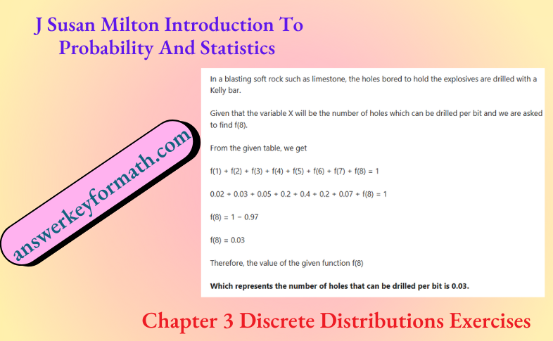
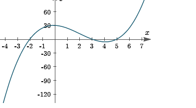
In a blasting soft rock such as limestone, the holes bored to hold the explosives are drilled with a Kelly bar.
Given that the variable X will be the number of holes which can be drilled per bit and we are asked to find the table for F.
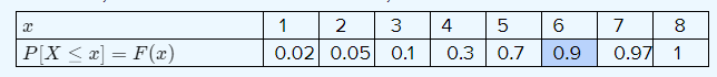
For the values x = 1,2,3,4,5,6,7,8, the value of F(x) will be
F(1) = P[X ≤ 1]
F(1) = f(1)
F(1) =0.02
F(2) = P[ X≤2 ]
F(2) = f(1) + f(2)
F(2) = 0.02+0.03
F(2) = 0.05
F(3) = P[X ≤ 3]
F(3) = f(1)+ f(2) + f(3)
F(3) = 0.02 + 0.03 + 0.05
F(3) = 0.1
F(4) = P[X ≤ 4]
F(4) = f(1) + f(2) + f(3) + f(4)
F(4) = 0.02 + 0.03 + 0.05 + 0.2
F(4) = 0.3
F(5) = P[X ≤ 5]
F(5) =f(1) + f(2) + f(3) + f(4) + f(5)
F(5)= 0.02 + 0.03 + 0.05 + 0.2 + 0.4
F(5) = 0.7
F(6) = P[X ≤ 6]
F(6) = f(1) + f(2) + f(3) + f(4) + f(5) + f(6)
F(6) = 0.02 + 0.03 + 0.05 + 0.2 + 0.4 + 0.2
F(6) = 0.9
F(7) = P[X ≤ 7]
F(7) = f(1) + f(2) + f(3) + f(4) + f(5) + f(6) + f(7)
F(7) = 0.02 + 0.03 + 0.05 + 0.2 + 0.4 + 0.2 + 0.07
F(7) = 0.97
F(8) = P[X ≤ 8]
F(8) = f(1) + f(2) + f(3) + f(4) + f(5) + f(6) + f(7) + f(8)
F(8) = 0.02 + 0.03 + 0.05 + 0.2 + 0.4 + 0.2 + 0.07 + 0.03
F(8) = 1
Therefore, the table for the value F will be
Introduction To Probability And Statistics Principles And Applications Chapter 3 Page 74 Exercise 6 Problem 8
In a blasting soft rock such as limestone, the holes bored to hold the explosives are drilled with a Kelly bar.
Given that the variable X will be the number of holes which can be drilled per bit and we are asked to find out the probability that a bit can be used to drill between three and five holes inclusive.
Using the F table, we get the probability of drilling between three and five holes inclusive
P [3 ≤ X ≤ 5] = P[X ≤ 5] − P[X > 3]
P [3 ≤ X ≤ 5] = P[X ≤ 5]−P[X ≤ 2]
P [3 ≤ X ≤ 5] = 0.7 − 0.05
P [3 ≤ X ≤ 5]= 0.65
Therefore, by using the table F, we get the probability of drilling between three and five holes inclusive is 0.65.
Chapter 3 Discrete Distributions Examples And Answers Susan Milton Page 75 Exercise 7 Problem 9
Let X denote the number of computer systems operable at the time of the launch.
Assume that each system is operable is 0.9.
We have to use the tree of table to find the density table.
Obtain the density table by
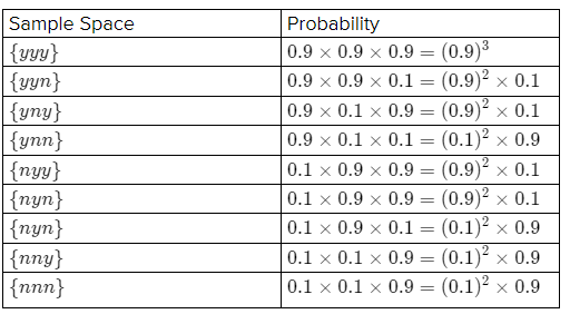
From the table sample space (S) is given below:
S={yyy,yyn,yny,ynn,nyy,nyn,nny,nnn}
Here, the probability of system is operable(y) is 0.9 and probability of system is not operable(n) is 0.1 =( 1−0.9).
Therefore, the probabilities are given below:
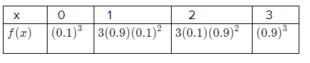
The density for X is given below
At x = 0, f(0) = (0.1)3
At x = 1
f(1) = (0.9)(0.1)2 + (0.9)(0.1)2 + (0.9)(0.1)2
f(1) = (0.9)(0.1)2 (1 + 1 + 1)
f(1) = 3(0.9)(0.1)2
At x = 2
f(2) = (0.1)(0.9)2 + (0.1)(0.9)2 + (0.1)(0.9)2
f(2) = (0.1)(0.9)2 (1 + 1 + 1)
f(2) = 3(0.1)(0.9)2
At x = 3
f(3) = (0.9)3
The density table for X is given below
Hence the equation x 2+ 6x in the form of (x + k)2 + his (x + 3)2 − 9.
Introduction To Probability And Statistics Principles And Applications Chapter 3 Page 75 Exercise 7 Problem 10
Let X denote the number of computer systems operable at the time of the launch.
Assume that each system is operable is 0.9.
There is a pattern to the probabilities in the density table.
In particular f(x) = k(x)(0,9)x (0.1)3 − x
Where k(x) gives the number of paths through the tree yielding a particular value for X.
We have to use F to find the probability that at least one system is operable at launch time.
We have to find the value of P(x ≥ 1).
Consider
⇒ P(x ≥ 1)
= 1−P(x < 1)
= 1−P(x ≤ 0)
= 1 − F(0)
From F table, the value of F(0) is 0.001.
Therefore
⇒ P(x ≥ 1)
= 1 − F(0)
= 1 − 0.001
= 0.999
Thus the probability that at least one system is operable at launch time is 0.999.
Hence using F table, the probability that at least one system is operable at launch time is 0.999.
Probability And Statistics J. Susan Milton Chapter 3 Solved Step-By-Step Page 75 Exercise 8 Problem 11
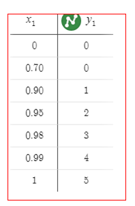
Given the function is
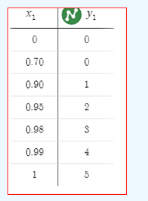
F(x) = \( \begin{cases}0 & x<0 \\ .70 & 0 \leq x<1 \\ .90 & 1 \leq x<2 \\ .95 & 2 \leq x<3 \\ .98 & 3 \leq x<4 \\ .99 & 4 \leq x<5 \\ 1.00 & x \geq 5\end{cases}\)
To draw the graph of this function.
Cumulative distribution
Let X be a discrete random variable with density f.
The cumulative distribution function for X, denoted by F is defined by F(x) = P[X≤x]for x real.
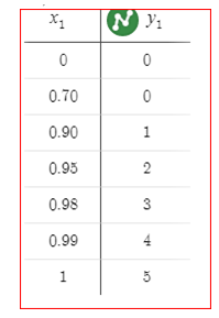
Yes. This function is called the step function.
Introduction To Probability And Statistics Principles And Applications Chapter 3 Page 75 Exercise 8 Problem 12
Given that
F(x) = \(\begin{cases}0 & x<0 \\ .70 & 0 \leq x<1 \\ .90 & 1 \leq x<2 \\ .95 & 2 \leq x<3 \\ .98 & 3 \leq x<4 \\ .99 & 4 \leq x<5 \\ 1.00 & x \geq 5\end{cases}\)
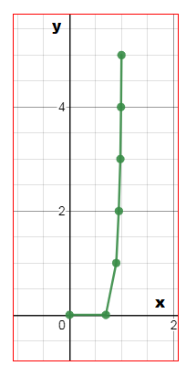
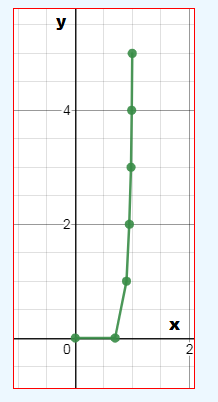
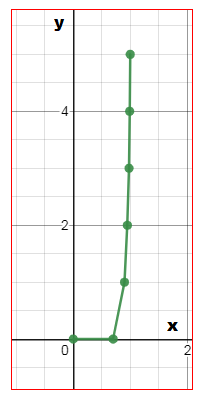
Need to determine that it is a continuous function
A function is said to be continuous as the values of x increases the function also increases.
Here I have attached an example graph which clearly explain that the function is continuous function.
Example of graph:
Similarly in our case also the graph increases as the value of x increases the function value also increases .
For example ,in our case consider any value to check that above said condition are satisfied.
1. f(a) Exists for any value of x
2. \(\lim _{x \rightarrow a} f(x)\) for each and every value of x from 0 to 5,the function exists.
3. \(\lim _{x \rightarrow a} f(x)\) = f(a) at last the function for every values
Therefore the given function is a continuous function.
Introduction To Probability And Statistics Principles And Applications Chapter 3 Page 75 Exercise 8 Problem 13
We need to find the \(\lim _{x \rightarrow \infty} F(x)\) and \(\lim _{x \rightarrow \infty}\) F(x)
Cumulative distribution
Let X be a discrete random variable with density f.
The cumulative distribution function for X, denoted by F, is defined by F(x) = P[X≤x] for x real.
The value of \(\lim _{x \rightarrow \infty} \) F(x) = 1 and the value of \(\lim _{x \rightarrow \infty}\) F(x) = 0
The value of \(\lim _{x \rightarrow \infty} \)F(x) = 1 and the value of \(\lim _{x \rightarrow \infty}\) F(x) = 0
Step-By-Step Guide To Discrete Distributions Exercises Chapter 3 Milton Page 76 Exercise 9 Problem 14
Given: In an experiment to graft Florida sweet orange trees to the root of a sour orange variety, a series of five trials is conducted.
Let X denote the number of grafts that fail.
The density for X is given in
To find – Find E[X]
We can find the E[X] by the following formula
E[X] = \(\sum_z x f(x)\)
So the expectation of the random variable X wil be as foliows:
E[X] = \(\sum_z x f(x)\)
E[X] = 0 × f(0) + 1 × f(1) + 2 × f(2) + 3 × f(3) + 4 × f(4) + 5 × f(5)
E[X] = 0 × 0.7 + 1 × 0.2 + 2 × 0.05 + 3 × 0.03 + 4 × 0.01 + 5 × 0.01
E[X] = 0 + 0.2 + 0.1 + 0.09 + 0.04 + 0.05
E[X] = 0.48
For the above two calculations we have used the R software.
Hence, from the above explanation value of E[X] is 0.48
Introduction To Probability And Statistics Principles And Applications Chapter 3 Page 76 Exercise 9 Problem 15
Given: In an experiment to graft Florida sweet orange trees to the root of a sour orange variety, a series of five trials is conducted.
Let X denote the number of grafts that fail.
The density for X is given in
TO find – Find μx
Since, we know that μx = E[X]
Therefore;So the expectation of the random variable X wil be as foliows:
E[X] = \(\sum_z x f(x)\)
E[X] = 0 × f(0) + 1 × f(1) + 2 × f(2) + 3 × f(3) + 4 × f(4) + 5 × f(5)
E[X] = 0 × 0.7 + 1 × 0.2 + 2 × 0.05 + 3 × 0.03 + 4 × 0.01 + 5 × 0.01
E[X] = 0 + 0.2 + 0.1 + 0.09 + 0.04 + 0.05
E[X] = 0.48
Hence, μx E[X] = 0.48
Hence, from the above explanation the value of μX is equal to 0.48.
Introduction To Probability And Statistics Principles And Applications Chapter 3 Page 76 Exercise 9 Problem 16
In an experiment to graft Florida sweet orange trees to the root of a sour orange variety, a series of five trials is conducted.
Let X denote the number of grafts that fail.
The density for X is
To Find μx
We can find the E[X2] by the following formula
E[X2] = \(\sum_z x f(x)\)
So the expectation of the random variable x will be as follows:
E[X2] = \(\sum_z x f(x)\)
f(x) =0 × f(0)+ 1 × f(1) + 22 × f(2) + 32 × f(3) + 42× f(4) + 52 × f(5)
f(x) = 0 × 0.7 + 1 × 0.2 + 4 × 0.05 + 9 × 0.03 + 16 × 0.01 + 25 × 0.01
f(x) = 0.210.210.27 + 0.1610.25
f(x) = 1.08
For the above two calculations we have used the R software.
Hence, from the above explanation the value of E[X2] is equal to 1.08.
Introduction To Probability And Statistics Principles And Applications Chapter 3 Page 76 Exercise 9 Exercise 17
Given: In an experiment to graft Florida sweet orange trees to the root of a sour orange variety, a series of five trials is conducted.
Let X denote the number of grafts that fail.
The density for X is
To find – Find σ X2.
We can find the σX = Var X by the following formula
Var X = E[X2] − (E[X])(E[X])2……………. (1)
Using the above & from Equation 1
VarX = E[X2]−(E[X])2
VarX = 1.08 − 0.482
VarX = 1.077
Hence, from the above explanation the value of the σX2 is equal to 1.077.
Introduction To Probability And Statistics Principles And Applications Chapter 3 Page 76 Exercise 10 Exercise 18
Given: The density for X,the number of holes that can be drilled per bit while drilling into limestone is given in
To find – Find E[X] and (E[X])2
In blasting soft rock such as limestone, the holes bored to hold the explosives are drilied with a Kelly bar.
This drill is designed so that the explosives can be packed into the hole before the drill is removed.
This is necessary since in soft rock the hole often collapses as the drill is removed. The bits for these drills must be changed fairly often.
Let X denote the number of holes that can be drilled per bit (a) We can find the E[X] by the following formula−
For the above two calculations we have used the
We can find the E[X2] by the following formula−
E[X2] \(-\sum_z x^2 f(x)\)
So the expectation of the random variable X wil be as follows:
E[X2] = \(-\sum_z x^2 f(x)\)
E[X2] = 1 × f(1) + 2 × f(2) + 32 ×f (3) + 42 × f(4)+ 52 × f(5) +62 × f(6)× 72 × f(7)+ 82 × f(8)
E[X2] = 1 × 0.02 + 4 × 0.03 + 9 × 0.05 + 16× 0.2+ 25 × 0.4+ 36 × 0.2+ 19 × 0.07 + 61 × 0.03
E[X2] = 0.02 + 0.12 + 0.45 + 3.2 + 10 + 7.2 + 3.43 + 1.92
E[X2] = 26.34
For the above two calculations we have used the R software.
Hence, from the above explanation the value of E[X] & E[X2] is equal to 4.96 & 26.34
Introduction To Probability And Statistics Principles And Applications Chapter 3 Page 76 Exercise 10 Exercise 19
Given: The density for X, the number of holes that can be drilled per bit while drilling into limestone is given in
To find – Find Var X and σx .
We can find the Var X by the following formula
Var X = E[X ]− (E[X])2
Using the above we get
Var X = E[X2] − (E[X])2
Var X = 26.34 − 4.962
Var X = 1.7384
Star dard deviation of X is giver by σx
= \(\sqrt{VarX}\)
Using the above we get
σx = \(\sqrt{VarX}\)
σx= \(\sqrt{1.7384}\)
σx= 1.318
Hence, from the above explanation the value of Var X and σx is 1.7384 & 1.318.
Exercise Solutions For Chapter 3 Susan Milton Discrete Distributions Page 76 Exercise 10 Exercise 20
Given : The density for X ,the number of holes that can be drilled per bit while drilling into limestone is g
To find – What physical unit is associated with σX?
The physical unit associated with σx is the number of holes that can be drilled per bit.
Hence, from the above explanation the physical unit associated with σx is the number of holes that can be drilled per bit.
Introduction To Probability And Statistics Principles And Applications Chapter 3 Page 76 Exercise 11 Problem 21
Given: Let X be a discrete random variable with density f.
Let c be any real number.
To find – Show that E[c] = c
As f(x) is the density of X given in the table, it should satisty \(\sum_{a l k} f(x)\) = 1
We can find the E[X] by the following formula-
E[X] = \(\sum_z x f(x)\)
So the expectation of c will be as follows:
E ∣c∣ = \(\sum_z c f(x)-c \sum_x f(x)\)
Hence, from the above explanation showed that E[c]= c
Introduction To Probability And Statistics Principles And Applications Chapter 3 Page 76 Exercise 11 Problem 22
Given: Let X be a discrete random variable with density f .
Let c be any real number.
To find – Show that E[cX] = cE[X]
As f(x)is the density of X given in the table, it should satisty
\(\sum_{a l k} f(x)\) = 1
We can find the E[X] by the following formula-
E[X] = \(\sum_z x f(x)\)
So the expectation of cX will te as follows:
E[cX] = \(\sum_z\)cxf(x)
E[cX] = c \(\sum_z x f(x)\)
E[cX] = cE[X]
Hence the above explanation we have showed that E[cX] = cE[X].
Introduction To Probability And Statistics Principles And Applications Chapter 3 Page 76 Exercise 12 Problem 23
Given: Use the rules for expectation
To find – To verify that Varc = 0, and Varc X = c{2} Var X for any real number c
We can find the Var X by the following formula
Var X = E[X]2 − (E[X])2
In order to get Var c we need to caculate E[c2] and E[c].
We can find the E[X] by the following formula
E[X] = \(\sum_z x f(x)\)
So the expectation of C will be as follows
E[c] = \(\sum_z x cf(x)\)
E[c] = c\(\sum_x f(x)\)
E[c] = c
We can find the E[X2] by the following formula
E[X2] = \(\sum_z c^2 f(x)\)
So the expectation of C will be as follows
E[c2] = \(\sum c^2 f(x)\)
E[c2] = c2\(\sum_z c x f(x)\)
E[c2] = c2
Using the above we get
Varc = E[c2 ]−(E[c2 ])
Varc= c2− c2 = 0
In orderto get Var(cX) , we need to calculate E[(cX)2 ]and F[cX].
We can find the E[cX] by the following formula
E[cX]= \(\sum_z c x f(x)\)
So the expectation of C will be as follows
E[c] =\(\sum_x c x f(x)\)
E[c] = c\(\sum_x f(x)\)
E[c] = cE[X]
We can find the F[X2]by the following formula
E[X2] = \(\sum_z x^2 f(x)\)
So the expectation of (cX)2 will be as follows:
E[c2X2] = \(\sum_z c^2 x^2 f(x)\)
E[c2X2] = c2 \(\sum_z x^2 f(x)\)
E[c2X2] = c2E[X2]
Using the above we get, Var cX = E[c2X2]− (E[cX])2 = e2 E[X2] − c2(E[X])2
= c2(E[X2] − (E[X])2)
= c2 Var X
Hence, from the above explanation by using the rules for expectation we verify that Varc = 0 and Varc X = c2 Var X for any real number c
Introduction To Probability And Statistics Principles And Applications Chapter 3 Page 76 Exercise 13 Problem 24
Given: Let X and Y be independent random variables with
E[X] = 3, E[X2] = 25, E[Y] = 10 and E[Y2] = 164
To find – Find E[3X + Y − 8]
Let X and Y be two independent random variables with
E[X] = 3, E[X2] = 25, E[Y] = 10 E[Y2] = 164
Using the above properties given in tip of expectation we can say:
E[3X + Y − 8] ⇒ E[3X] + E[Y] + E[−8] (Using rule 3)
E [3X + Y − 8] = 3E[X] + E[Y] + E[−8] (Using rule 2)
E [3X + Y − 8] = 3E[X] + E[Y] − 8
E [3X + Y − 8] = 3 × 3 + 10 − 8
E [3X + Y − 8] = 9 + 10 − 8
E [3X + Y − 8] = 11
So we find E [3X + Y − 8] = 11
Hence, from the above explnation the value of E[3X+Y−8]=11.
Page 76 Exercise 13 Problem 25
Given: Let X and Y be independent random variables with E[X]= 3, E[X2 ] = 25, E[Y] = 10 and E[Y2] = 164
To find – Find E [2X − 3Y + 7].
We will use some properties of expectation.
LetX and Y be random variables and C be any real number.
1. E[c] = c (The expected value of any constant is that constant)
2. E[cX] = cE ∣X∣ (Constants can be fectored from expectat ons.)
3. E[X + Y] = E[X] − E[Y] (The expected value of a sum is equal to the sum of the expected values.)
Using the above properties of expectation we can say-
E[2X−3Y+7]= E[2X] − E[−3Y] + E[7] (Using rule 3)
E[2X − 3Y + 7]= 2E[X]−(−3)E[Y]+E[7]
E[2X − 3Y + 7]= 2E[X]−(−3)E[Y] + 7 (Using rule 1)
E[2X − 3Y + 7]= 2 × 3 − 3 × 10 + 7
E[2X − 3Y + 7]= 6 − 30 + 7
E[2X − 3Y + 7]= −17
So we find E[2X − 3Y + 7] = −17
Hence, from the above explanation the value of E[2X − 3Y + 7] = −17
Introduction To Probability And Statistics Principles And Applications Chapter 3 Page 76 Exercise 15 Problem 26
Let X and Y be independent random variables with E[X] = 3
E[X2] = 25, E[Y] = 10 and E[Y2] = 164.
We have to find VarX.
From the formulae of variance we know that
Var X = E[X2] − (E[X])2
Using the above we get
Var X = E[X2] − (E[X])2
Var X= 25−32
Var X= 25−9
Var X= 16
Hence the value of V ar X is 16.
Page 76 Exercise 15 Problem 27
Let X and Y be independent random variables with E[X] = 3, E[X2 ] = 25
,E[Y] = 10 and E[Y2 ] =164.
We have to find σx.
Standard deviation of X is given by σx
σx= \(\sqrt{Var X}\)
σx= \(\sqrt{16}\)
σx= 4
Hence the value of σx .is 4..
Introduction To Probability And Statistics Principles And Applications Chapter 3 Page 77 Exercise 16 Problem 28
Given: The function f is defined by f(x) = (1/2)−∣x∣
Where x = ±1,± 2,± 3,± 4,….
To be found: Verify that the given function is the density for a discrete random variable X
We have, the function f is defined by f(x) = (1/2)2−∣x∣
where x = ± 1,± 2, ± 3,± 4,….
Using the first condition for all, we get
We know, x is a real number
⇒ 2 − ∣x∣ ≥ 0
⇒ f(x) ≥ 0
Using the second condition to verify, we get
⇒ \(\sum_x f(x)\) =\(\sum_x \frac{1}{2} 2^{-|x|}\)
⇒ \(\sum_x f(x)\) = \(\sum_x \frac{1}{2} 2^{-|x|}\) = \(\ldots+\sum_x \frac{1}{2} 2^{-|-2|}+\sum_x \frac{1}{2} 2^{-|-1|}+\sum_x \frac{1}{2} 2^{-|1|}+\sum_x \frac{1}{2} 2^{-|2|}+\)………
⇒ \(\sum_x f(x)\) =\(\sum_x \frac{1}{2} 2^{-|x|}\)
= 2 − 1 + 2 − 2 + 2 − 3 +…………..
⇒ \(\sum_x f(x)\) = \( \frac{2^{-1}}{1-2^{-1}}\)
⇒ \(\sum_x f(x)\) = \(\sum_x \frac{1}{2} 2^{-|x|}\)
Finally, we get the required condition,\(\sum_x f(x)\) = 1
Hence, verified that the given function
f(x) = (1/2)2−∣x∣, where x = ± 1, ± 2, ± 3, ± 4,…. is the density for a discrete random variable X.
Hence, verified that the given function f(x)=(1/2)2−∣x∣ , where x = ±1, ± 2, ± 3, ± 4,…. is the density for a discrete random variable X.
Introduction To Probability And Statistics Principles And Applications Chapter 3 Page 77 Exercise 16 Problem 29
Given: The function f is defined by f(x) = (1/2)2−∣x∣
where x = ±1,± 2, ± 3,± 4,….
Let g(X) = (−1)∣X∣−1 [2∣x∣/ 2 ∣X∣ − 1)]
To be found: Show that \(\sum_{\text {all }} x(x) f(x)<\infty\)
We have, g(X) =[(2 ∣X∣ /2 ∣X∣ − 1)] and f(x) = (1/2)2−∣x∣
Now, substituting the above values and expanding the series, we get \(\sum_{\text {all }} x g(x) f(x)\)
⇒ \(\sum_{a l l} x(x) f(x)=\sum_x(-1)^{|x|-1}\left[\frac{2^{|x|}}{(2|x|-1)}\right]\)\(\frac{1}{2} 2^{-|x|}\)
⇒ \(\sum_{a l l}{ }_x g(x) f(x)=\sum_x(-1)^{|x|-1}\left[\frac{2^{|x|}}{(2|x|-1)}\right] \frac{1}{2}\)
\(\Rightarrow \sum_{\text {all }} x g(x) f(x)=\sum_x^{\infty}(-1)^{x-1}\left[\frac{2^x}{(2 x-1)}\right] \frac{1}{2}\)
Expanding the series, we get a final alternating series which converges
\(\Rightarrow \sum_{\text {all }}{ }_x g(x) f(x)=1-\frac{1}{3}+\frac{1}{5}-\frac{1}{7}+\ldots \ldots+\infty\)
Hence , proved that \(\sum_{a l l} x g(x) f(x)\)
By the method of expansion, it is shown that \(\sum_{a l l} x g(x) f(x) \) <∞