
J. Susan Milton Introduction To Probability And Statistics Principles And Applications Chapter 4 Continuous Distributions
Introduction To Probability And Statistics Chapter 4 Exercises Solutions Page 127 Exercise 1 Problem 1
Given:
The function f(x) = kx where 2 ≤ x ≤ 4
To find – The value of k
Method: The method here used is probability and continuous random variable.
The function f(x) = kx.
For, 2 ≤ x ≤ 4 variable.
Assume x = 3.
f(3) = 3k
Consider f(3) = 1 for the function f(x).
1 = 3k
k = \(\frac{1}{3}\)
Hence, it is verified that the value of k is k = \(\frac{1}{3}\)
Read and Learn More J Susan Milton Introduction To Probability And Statistics Solutions
J. Susan Milton Introduction To Probability And Statistics Principles And Applications Chapter 4 Page 127 Exercise 1 Problem 2
Given:
The function f(x) = kx
Where 2 ≤ x ≤ 4.
To find:
Find the value of probabilities of P(2.5 ≤ X ≤ 3).
Method: The method here used is probability and continuous random variable.
The function f(x) = kx where 2 ≤ x ≤ 4
Substitute x = 3
f(3) = 3k
The function of P[2.5≤X≤3]
Here, there is no function that occurs between the X = 2.5 and X = 3 X.
Hence, it is verified that the function f(x) is not possible for the values P(2.5 ≤ X ≤ 3).
J. Susan Milton Introduction To Probability And Statistics Principles And Applications Chapter 4 Page 127 Exercise 1 Problem 3
J. Susan Milton Chapter 4 Continuous Distributions Answers Page 127 Exercise 1 Problem 4
Given:
The function f(x) = kx
where 2 ≤ x ≤ 4.
To find – Find the probability of P(2.5 < X ≤ 3)
Method: The method here used is probability and continuous random variable.
The function f(x) = kx
For P (2.5 < X ≤ 3)
The equation is, f(x) = 3k
Assume k = 2
The function
f(x) = 3 × 2
f(x) = 6
Hence, it is verified that the function f(x) at P(2.5 < X ≤ 3) is f(x) = 6
J. Susan Milton Introduction To Probability And Statistics Principles And Applications Chapter 4 Page 128 Exercise 2 Problem 5
Given:
The function f(x) = \(\left(\frac{1}{10}\right) e^{\frac{-x}{10}}\)
To find – The function is a continuous random variable
Method : The method used is a probalility and continuous random variable
The given function f(x) =\(\left(\frac{1}{10}\right) e^{\frac{-x}{q p}}\)
Substitute 1 or x
f(1) \( = \frac{1}{10} e^{\frac{-x}{10}}\)
f(1) = 0.0904
Hence, it is verified that the density of the function is f(1) = 0.0904
Solutions To Continuous Distributions Exercises Chapter 4 Susan Milton Page 128 Exercise 2 Problem 6
Given:
The function f(x)= \(\frac{1}{10} e^{\frac{-x}{10}}\)
To find – Find the density at 7 minutes
Method: The method used here are probability and continuous random variable.
The given function
f(x) = \(\frac{1}{10} e^{\frac{-x}{10}}\)
For the density of 7 minutes
f(7) = \(\frac{1}{10} e^{\frac{-7}{10}}\)
f(7) = 0.0496
Hence, it is verified that the density of the function at 7 minutes is f(7) = 0.0496
J. Susan Milton Introduction To Probability And Statistics Principles And Applications Chapter 4 Page 128 Exercise 2 Problem 7
Given:
The function f(x) = \(\frac{1}{10} e^{\frac{-x}{10}}\)
To find – The probability of density of call last between 1 to 2 minutes.
Method: The method used here is probability and continuous random variable.
The given function is.
f(x) = \(\)
For the call last one minute
f(1) = \(e^{\frac{-1}{10}}\)
f(1) = 0.0904
For the call lasts two minutes
f(2) = 0.1 × \(e^{\frac{-2}{10}}\)
f(2) = 0.0607
The probaability of the call lasts one minuteto two minutes, the density of the function gradually increases to show the calls gain more and more density by increasing the call time.
Hence, it is verified that the call lasts from one to two minutes then the density of the call is also increasing.
J. Susan Milton Introduction To Probability And Statistics Principles And Applications Chapter 4 Page 128 Exercise 3 Problem 8
Given:
The graph of bird moving in θ.
To find – The angle of the bird moving
Method: The method used in this problem is probability, continuous random variable, and graphical method.
Let the function f for the interval [0,2Π].
f(θ)\(=\int_0^{2 \Pi} \theta\)
Reduce the equation.
f(θ) = 2Π − 0
f(θ) = 2Π
Hence, it is verified that the density of the function f with the interval [0,2Π] is f(θ) = 2Π
Chapter 4 Continuous Distributions Examples And Answers Susan Milton Page 128 Exercise 3 Problem 9
Given:
The graph of moving bird denoted in θ.
To find – Sketch the graph of the moving bird in uniform motion with interval [0,2Π].
Method: The method used in this problem is probability, continuous random variable, and graphical method.
The function of the moving bird in uniform distribution interval [0,2Π].
Let \(=\int_0^{2 \Pi} \theta\)
Reduce the equation.
f(θ) = Π + Π
f(θ) = 2Π
The graph of the moving bird.
Hence, it is verified that the graph of a uniform distribution over the interval.

J. Susan Milton Introduction To Probability And Statistics Principles And Applications Chapter 4 Page 128 Exercise 3 Problem 10
Given:
The function f of moving bird in the angle θ.
To find – Sketch the graph of the function fin the interval [0,2Π].
Method: The method used in this problem is a probability, continuous random variable, and graphical method
Graph the function f and shade the orient within \(\frac{\Pi}{4}\)radians of home.
The graphs shows, the bird flying in the direction of \(\frac{\Pi}{4}\) radians from home in the straight direction from home.
Hence, it is verified that the

J. Susan Milton Introduction To Probability And Statistics Principles And Applications Chapter 4 Page 128 Exercise 3 Problem 11
Given:
The function f mof the interval [0,2Π].
To find – Find the probability of the function f with the orient within the
\(\frac{\Pi}{4}\) radians of home.
Method: The method used in this problem is a probability, continuous random variable, and graphical method.
The function for orient within the \(\frac{\Pi}{4}\) radians of the home .
f(θ)\( =\int_0^{2 \Pi} \theta+\frac{\Pi}{4}\)
Reduce the equation.
f(θ) = \(2 \Pi+\frac{\Pi}{4}\)
f(θ) = \(\frac{9 \Pi}{4}\)
Hence, it is verified that the possibilities of the moving bird within the
\(\frac{\Pi}{4}\) radians of home is \(=\frac{9 \Pi}{4}\)
Probability And Statistics J. Susan Milton Chapter 4 Solved Step-By-Step Page 129 Exercise 4 Problem 12
Given:
The graph of the probabilities.
To find: Show probabilities in terms of the cumulative distribution function F.
Method: The method used in this problem is a probability, continuous random variable, and cumulative distribution function.
The graph f(x) of the cumulative distribution function F(x) has the possible intervals of 0 ≤ x ≤ 20.
For graph A
F(x) = \(\int_0^{20} x+1 d x\)
Reduce the equation.
F(x) = 20 + 1−(0 + 1)
F(x) = 20
The probability at graph A X≤ 5
Similarly, for the graph B, C, D, and E
F(x)= \(\int_0^{20} x+1 d x\)
Reduce the equation
F(x) = 20 + 1−(0 + 1)
F(x) = 20
The probability of graph B, X > 5.
The probability of graph C, X = 10.
The probability of graph D, 5 ≤ X < 10.
The probability of graph E, 5 < X < 10
Hence, it is verified.
The probability of the graph A, X ≤ 5.
The probability of the graph B, X > 5.
The probability of the graph C, X = 0.
The probability of the graph D, 5 ≤ X < 10.
The probability of the graph E, 5 < X < 10.
J. Susan Milton Introduction To Probability And Statistics Principles And Applications Chapter 4 Page 129 Exercise 5 Problem 13
Given:
The function f(x) = kx where 2 ≤ x ≤ 4.
To find – Find the cumulative function of F(x).
Method:
The method used in this problem is a probability, continuous random variable, and cumulative distribution function.
The given function is f(x) = kx where 2 ≤ x ≤ 4.
The cumulative distribution function is
F(X) = \(\int_2^4(k x) d x\)
Reduce the equation.
F(X) = 4k − 2k
F(X) = 0 2k
Hence, it is verified that the cumulative distribution function of F(x) = 2k.
Step-By-Step Guide To Continuous Distributions Exercises Chapter 4 Milton Page 129 Exercise 5 Problem 14
Given:
The cumulative distribution function , F(X) = \(=\int_2^4 k X d X\)
To find – Find the cumulative distribution function, P[2.5 ≤ X ≤ 3].
Method: The method used in this problem is a probability, continuous random variable, and cumulative distribution function.
The given function.
F(X) = \(\int_2^4 k x d x\)
The cumulative distribution function for the interval P[2.5 ≤ X ≤ 3].
F(X) = \(\int_{2.5}^3 k x \mathrm{dx}\)
Reduce the equation.
F(X) = 3k − 2.5k
F(X) = 0.5k
Hence, it is verified that the cumulative distribution function of the interval P[2.5 ≤ X ≤ 3] is F(X) = 0.5k
J. Susan Milton Introduction To Probability And Statistics Principles And Applications Chapter 4 Page 129 Exercise 5 Problem 15
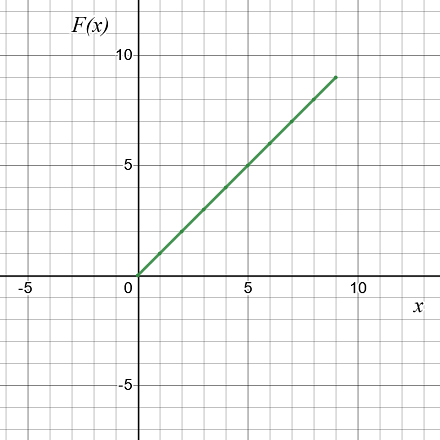
Given:
The function F with limits \(\lim _{n \rightarrow \infty} F(x)\) and \(\lim _{n \rightarrow \infty} F(x)\).
To find – Draw the graph of a function with limits \lim _{n \rightarrow \infty} F(x)
Method: The method used in this problem is a probability, continuous random variable, and cumulative distribution function.
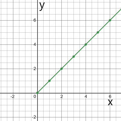
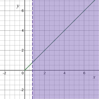
The graph of the cumulative distribution function
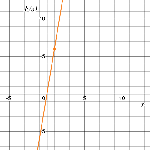
Here, the graph of the function shows the function F is the increasing function.
This function is a non-decreasing function up to the interval \(\lim _{n \rightarrow \infty} F(x)\) and \(\lim _{n \rightarrow \infty} F(x)\) is possible in the graph of the function.
Hence, it is verified that graph of the cumulative distributive function Fand the function is non-decreasing.

J. Susan Milton Introduction To Probability And Statistics Principles And Applications Chapter 4 Page 129 Exercise 6 Problem 16
Given:
The function f(x) = \(\frac{1}{b-a}\)
To find – Find the uniform distribution over the interval (a,b).
Method: The method used in this problem is a probability, continuous random variable, and cumulative distribution function.
The function f(x) = \(\frac{1}{b-a}\)
The uniform distribution over the interval (a,b).
The cumulative distribution function
f(x) = \(\int_a^b \frac{1}{b-a} d x\)
f(x) = \(\left[\frac{x}{b-a}\right]_a^b\)
f(x) = \(\frac{b}{b-a}-\frac{a}{b-a}\)
f(x) = \(\frac{b-a}{b-a}\)
f(x) = 1
Hence, it is verified that the uniform distribution over the interval (a,b) is f(x)=1
Exercise Solutions For Chapter 4 Susan Milton Continuous Distributions Page 129 Exercise 7 Problem 17
Given: The function f(θ) \(=\int_0^{2 \Pi} \theta d \)
To find –
Find the uniform distribution of f.
Method – The methods used here are a probability, cumulative random variable, and uniform distribution.
The function f(θ) \(=\int_0^{2 \Pi} \theta d \theta\)
For the cumulative distribution function, θ = Π.
f(θ) \(=\int_0^{2 \Pi} \theta d \theta\)
f(θ) = 2 Π
Hence, it is verified that the uniform distribution of cumulative function is f(θ) = 2Π.
J. Susan Milton Introduction To Probability And Statistics Principles And Applications Chapter 4 Page 129 Exercise 7 Problem 18
Given:
The function f(θ) = \(\int_0^{2 \Pi} \theta d \)
To find – Graph the function F and F is non-decreasing or not.
Method: The method used here is a probability, cumulative distributive function and uniform distribution.
The function.
f(θ) = \(\int_0^{2 \Pi} \theta d \)
Reduce by uniform Distribution.
F(θ) = [θ2]02π
F(θ) = 4Π2
The graph of the function
Hence, it is verified that the uniform function is F(θ)=4Π2 and the function is non-decreasing. The graph of the function F

J. Susan Milton Introduction To Probability And Statistics Principles And Applications Chapter 4 Page 129 Exercise 8 Problem 19
Given:
The function f(x)=\(\frac{1}{10} e^{\frac{-x}{10}}\).
To find – Find the Cumulative distribution f.
Method: The methods used here are probability, cumulative distribution function.
The function
f(x) = \(\frac{1}{10} e^{\frac{-x}{10}}\).
For the interval P[1 ≤ X ≤ 2] .
The cumulative distribution function X = 1
f(1) = \(\frac{1}{10} e^{\frac{-1}{10}}\)
f(1) = 0.906 × 0.1
f(1) = 0.906
The cumulative distribution function X = 2
f(1) = \(\frac{1}{10} e^{\frac{-2}{10}}\)
f(2) = 0.1 × 0.818
f(2) = 0.0818
Hence, it is verified that the continuous random variable has only one possibilities of probability, but the cumulative distribution function has two probability values.
J. Susan Milton Introduction To Probability And Statistics Principles And Applications Chapter 4 Page 129 Exercise 9 Problem 20
Given:
The function f(x) = \(\frac{1}{\ln 2} \frac{1}{x}\).
To find – Find the cumulative distribution of function f.
Methods: The methods used here is the probability, cumulative distribution function
The given function f(x)= \(\frac{1}{\ln 2} \frac{1}{x}\)
The cumulative distribution of interval P[30 ≤ X ≤ 40].
For X = 30
f(x) = \(\frac{1}{\ln 2} \frac{1}{30}\)
f(x) = 1.44 × 0.33
f(x) = 0.475
Hence, it is verified that the cumulative distributive function of function f is f(x) = 0.475
J. Susan Milton Introduction To Probability And Statistics Principles And Applications Chapter 4 Page 129 Exercise 10 Problem 21
Given: The function
F(x) = \(\left\{\begin{array}{c}0, \mathrm{X}<-1 \\X+1,-1 \leq x \leq 0 \\1, x>0\end{array}\right.\)
To find – Find the cumulative distribution function.
Method: The methods used here are probability and cumulative distributive function.
The given function.
F(x) = \(\left\{\begin{array}{c}
0, \mathrm{X}<-1 \\
X+1,-1 \leq x \leq 0 \\
1, x>0
\end{array}\right.\)
The cumulative distribution function.
For, X < − 1.
F(x) = 0
For, −1 ≤ x ≤ 0.
F(x) = 1
For, x > 0.
F(x) = 1
Hence, it is verified that the cumulative distributive function is F(x)=1 and the function is non-decreasing for the limit \(\lim _{x \rightarrow-\infty} F(x)\) = 0 and \(\lim _{x \rightarrow-\infty} F(x)\) = 1.
J. Susan Milton Introduction To Probability And Statistics Principles And Applications Chapter 4 Page 129 Exercise 10 Problem 22
Given:
The function F(x)= \(\left\{\begin{aligned}
0, \mathrm{X} & \leq 0 \\
x^2, 0<x & \leq \frac{1}{2} \\
\frac{1}{2} x, \frac{1}{2}<x & \leq 0 \\
1, \mathrm{x} & >1
\end{aligned}\right.\)
To find – Find the cumulative distribution function.
Method: The methods used here are probability, cumulative distributive function.
The given function.
F(x) = \(\left\{\begin{array}{r}
0, \mathrm{X} \leq 0 \\
x^2, 0<x \leq \frac{1}{2} \\
\frac{1}{2} x, \frac{1}{2}<x \leq 0 \\
1, \mathrm{x}>1
\end{array}\right.\)
For, x ≤ 0.
F(x) = 0
For, 0 < x ≤ \(\frac{1}{2}\)
F(x) = \(\frac{1}{4}\)
For, \(\frac{1}{2}\) <x≤0.
F(x)= \(\frac{1}{4}\)
For, x > 1.
F(x) = 1
Hence, it is verified that the cumulative distributive function is F(x)= \(\frac{1}{4}\) and function is ono-decreasing with the limit F(x) = 0.
J. Susan Milton Introduction To Probability And Statistics Principles And Applications Chapter 4 Page 130 Exercise 11 Problem 23
Given:
The function f(x) = \(\frac{1}{6}\) (x) where 2 ≤ x ≤ 4.
To find – Find the function E(X) f(x) =\(\frac{1}{6}\)(x).
Method:
The method used here is probability, cumulative distributive function.
The function f(x)= \(\frac{1}{6}\)
The uniform distribution.
For, 2 ≤ x ≤ 4.
E(X) = \(\int_2^4 f(x) d x\)
Reduce the equation.
E(X) = \(\int_2^4 \frac{1}{6}(x) d x\)
E(X) = \(\frac{1}{6}\left[x^2\right]_2^4\)
E(X) =\(\frac{1}{6}\)(16 – 4)
E(X) = \(\frac{1}{6}\)(12)
E(X) = 2
Hence, it is verified that the uniform distribution of the function f(x) = \(\frac{1}{6}\) (x) E(x) = 2
J. Susan Milton Introduction To Probability And Statistics Principles And Applications Chapter 4 Page 130 Exercise 11 Problem 24
Given:
The function f(x) = \(\frac{1}{6}\) (x) where 2 ≤ x ≤ 4.
To find –
Find E(X2).
Method: The methods used here are probability, Cumulative distributive function, and Uniform distribution.
The function f(x) = \(\frac{1}{6}\) (x).
The cumulative distribution of function.
E(X2) = \(\int_2^4(f(x))^2 d x\)
Reduce the equation.
E(X2) = \(\int_2^4 \frac{1}{36}\left(x^2\right) d x\)
E(X2) = \(\left.\frac{1}{36} \frac{x^3}{3}\right]_2^4\)
E(X2) = \(\left(\frac{16}{27}\right)-\left(\frac{2}{27}\right)\)
Hence, it is verified the uniform distribution of the function f(x) = \(\frac{1}{6}x\) is E(X2) =\(\frac{14}{7}\).
Page 130 Exercise 12 Problem 25
Given:
The function f(x) = \(\frac{1}{10} e^{\frac{-x}{10}}\) where x>0.
To find – Find the moment generating function MX(t).
Method: The method used here is the cumulative distribution function and the uniform distribution.
The function f(x) = \(\frac{1}{10} e^{\frac{-x}{10}}\) where x>0
The expression for moment generating function MX(t)
MX(t)= E [ext]
Reduce the equation.
Mx(t) = \(\int_1^{\infty} e^{t x} \frac{1}{10} e^{\frac{-x}{10}} d x\)
Mx(t) = 0.1 [\(\left[e^{t x} \frac{1}{10} e^{\frac{-x}{10}}\right]_1^{\infty}\)
MX(t) = 0.1 \(\left[e^{t x-\frac{x}{10}}\right]_1^{\infty}\)
Mx(t) = 0.1 \(\left[e^{t-\frac{1}{10}}-e^{\infty}\right]\)
Mx(t) = 0.1 \(0.1\left[e^{t-0.1}-\infty\right]\)
Mx(t) = ∞
Hence, it is verified that the moment generating function is Mx(t) = ∞.
J. Susan Milton Introduction To Probability And Statistics Principles And Applications Chapter 4 Page 130 Exercise 12 Problem 26
Given:
The function f(x)= \(\int_1^{\infty} e^{t x} \frac{1}{10} e^{\frac{-x}{10}} d x\) where x>0.
To find – Find the average length of such a call with the moment generating function.
Method: The method used here is the cumulative distribution function and the uniform distribution.
The function f(x)= \(\int_1^{\infty} e^{t x} \frac{1}{10} e^{\frac{-x}{10}} d x\).
The Expression for the moment generating function.
Mx(t) = E[etX]
Mx(t) = \(0.1\left[e^{t-\frac{1}{10}}-\infty\right]\)
For the average length of a call, assume t = 1.
Mx(1) = \(0.1\left[e^{t-\frac{1}{10}}-\infty\right]\)
Mx(t) = \(0.1\left[e^{t-\frac{1}{10}}-\infty\right]\)
Mx(t) = ∞
Hence, it is verified that the average length of such a call in moment generating function is Mx(t) = ∞.