J.Susan Milton Introduction To Probability and Statistics Principles And Applications Chapter 5 Joint Distributions Exercises

J.Susan Milton Introduction To Probability And Statistics Principles And Applications Chapter 5 Joint Distributions 

 

Page 169  Exercise 1  Problem 1

In Given problem, is a hypergeometric distribution.

Hypergeometric distribution: A random variable X has a hypergeometric distribution with parameters N,n and r if its density is given by

f(x) = \(\frac{\left(\begin{array}{l}
r \\
x
\end{array}\right)\left(\begin{array}{l}
N-r \\
n-x
\end{array}\right)}{\left(\begin{array}{l}
N \\
n
\end{array}\right)}\)

Max [0,n−(N−r)] ≤ x ≤ min(n,r)

Given table

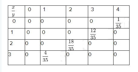
Find the probability for hypergeometric function

Using given statement to get a required probability such as, N = 7,r = 3

P(X = x) = \(\frac{\left(\begin{array}{l}
r \\
x
\end{array}\right)\left(\begin{array}{l}
N-r \\
n-x
\end{array}\right)}{\left(\begin{array}{l}
N \\
n
\end{array}\right)}\)

Putx = 0 in above equation

P(X = x) = \(\frac{\left(\begin{array}{l}
3 \\
0
\end{array}\right)\left(\begin{array}{l}
7-3 \\
4-0
\end{array}\right)}{\left(\begin{array}{l}
7 \\
4
\end{array}\right)}\)

P(X = x) = \(\frac{1}{35}\)

Therefore, the probability for a hypergeometric function value is \(\frac{1}{35}\) and the table values are verified.

 

Page 169  Exercise 1  Problem 2

Using given table values for determine the marginal density of the function.

If two random variables with joint density${{f}_{XY}}$,then the marginal density for X denoted as fXgiven by

f_x(x) =  y∑ f_xy(x,y)

\(f_X(x)=\sum_y f_{X Y}(x, y)\)

 

 The marginal density for Y denoted as

\(f_Y(y)=\sum_y f_{X Y}(x, y)\)

 

Using Given table to get a marginal density

Find the sum of all values to get the marginal density for a hypergeometric distribution.

Determine the marginal density of X and Y

Hence, the marginal density was obtained and the variable Y is the Continuous Random Variable.

Therefore, the marginal density was obtained and the variable Y is the Continuous Random Variable.

 

Page 169  Exercise 1 Problem 3

If two random variables are independent then it satisfies the following conditions,

​1. P(x/y) = P(x)

2. P(x ∩ y) = P(x) ∗ P(y)
​
Also, the joint distribution of a function is f_xy (x,y) = f_x (x) f_y(y)

Two random variables are independent, if the value of one variable does not change the probability value of another variable.

Therefore, If two random variables for independent then satisfies a condition 1. P(x∣y) = P(x) , 2. P(x∩y) = P(x)∗ P(y)

​

Page 169   Exercise 2   Problem 4

Given problem, f_xy(x,y) = 1/n²

If determine a function has to be joint density function satisfies the below condition,\(\sum_x \sum_y f_{X Y}(x, y)\) = 1

The values of X and Y between

​x = 1,2,3 ,…., n

y = 1,2,3, …., n

​Given: f_xy(x,y) = 1/n²

Find joint density function

\(\sum_x \sum_y f_{X Y}(x, y)=\sum_{x=1}^n \sum_{y=1}^n \frac{1}{n^2}\)

 

\(\sum_x \sum_y f_{X Y}(x, y)=\frac{1}{n^2} \sum_{x=1}^n \sum_{y=1}^n 1\)

 

\(\sum_x \sum_y f_{X Y}(x, y)=\frac{n}{n^2} \sum_{y=1}^n 1\)

 

\(\sum_x \sum_y f_{X Y}(x, y)=\frac{n}{n^2}(n)\)

 

\(\sum_x \sum_y f_{X Y}(x, y)\) = 1

Hence, a given function is discrete joint density function and the condition is satisfied.

Therefore, the function is a discrete joint density function and the condition x \(\sum_x \sum_y f_{X Y}(x, y)\) = 1 is satisfied.

 

Page 169  Exercise 2  Problem 5

Given problem, fxy(x,y) = 1/n²

If determine a function has to be joint density function satisfies the below condition,\(\sum_x \sum_y f_{X Y}(x, y)\)= 1

The values of X and Y between

​x = 1,2,3, …., n

y = 1,2,3, …., n

Given: fxy(x,y)=1/n²

Find joint density function

Using given function to get a marginal density

Find the marginal density of X

\(f_X(x)=\sum_y f_{X Y}(x, y)\)

 

\(f_X(x)=\sum_1^n \frac{1}{n^2}\)

 

\(f_X(x)=\frac{1}{n^2} \sum^n 1\)

 

\(f_X(x)=\sum_1^n \frac{1}{n^2}\)

 

\(f_X(x)=\frac{1}{n^2} \sum_1^n 1\)

 

Determine the marginal density of Y

\(f_Y(y)=\sum_1^n \frac{1}{n^2}\)

 

\(f_Y(y)=\frac{1}{n^2} \sum_1^n 1\)

 

 \(f_Y(y)=\frac{1}{n^2}(n)\)

 

 \(f_Y(y)=\frac{1}{n}\)

Therefore, the marginal densities of a given function both X and Y is  \(\frac{1}{n}\)

 

Page 169  Exercise 2  Problem 6

If two random variables are independent then it satisfies the following conditions,

​1. P(x∣y) = P(x)

2. P(x ∩ y) = P(x) ∗ P(y)
​
Also, the joint distribution of a function is

fxy(x,y) = f_x(x) f_y(y)

Two random variables are independent, if the value of one variable does not change the probability value of another variable.

Given problem,{{f}{XY}}(x,y) = 1/n²

The marginal densities of a given function both X
and Y is \(f_Y(y)=\frac{1}{n}\).

Hence, the values are independent.

Therefore, the given function marginal densities of both X and Y is \(f_Y(y)=\frac{1}{n}\) and independent.

 

Page 169  Exercise 3  Problem 7

Given problem ,f_xy(x,y) = 2/n(n+1)

If determine a function has to be joint density function satisfies the below condition \(f_Y(y)=\frac{1}{n}\).

The values of X and Y between

​x = 1,2,3,….,n

y = 1,2,3,….,n
​
Given: f_xy (x,y) = 2/n(n + 1)

Find joint density function

\(\sum_{y=1}^n \sum_{x=1}^n f_{X Y}(x, y)=\sum_{y=1}^n \sum_{x=1}^n \frac{2}{n(n+1)}\)

 

\(\sum_{y=1}^n \sum_{x=1}^n f_{X Y}(x, y)=\frac{2}{n(n+1)} \sum_{y=1}^n \sum_{x=1}^n \)

 

Sum of first n integers is given by \(\frac{n(n+1)}{2}\)

\(\sum_{y=1}^n \sum_{x=1}^n f_{X Y}(x, y)=\frac{2}{n(n+1)} \times \frac{n(n+1)}{2}\)

 

\(\sum_{y=1}^n \sum_{x=1}^n f_{X Y}(x, y)\) =  1

 

Hence, a given function is discrete joint density function and the condition is satisfied.

Therefore, the function is a discrete joint density function and the condition \(\sum_{y=1}^n \sum_{x=1}^n f_{X Y}(x, y)\)= 1 is satisfied.

 

Page 169  Exercise 3  Problem 8

Given problem, f_xy (x,y) = 2/n(n + 1)

If determine a function has to be joint density function satisfies the below condition \(f_Y(y)=\frac{1}{n}\).

The values of X and Y between

​x = 1,2,3,….,n

y = 1,2,3,….,n

Using given function to get a marginal density

Find the marginal density of X,

\(f_X(x)=\sum_y f_{X Y}(x, y)\)

 

\(f_X(x)=\sum_{y=1}^n \frac{2}{n(n+1)}\)

 

\(f_X(x)=\frac{2}{n(n+1)} \sum_{y=1}^n 1\)

 

\(f_X(x)=\frac{2}{n(n+1)}(n)\)

 

\(f_X(x)=\frac{2}{(n+1)}\)

 

Determine the marginal density of Y

\(f_X(x)=\sum_y f_{X Y}(x, y)\)

 

\(f_X(x)=\sum_{y=1}^n \frac{2}{n(n+1)}\)

 

\(f_X(x)=\frac{2}{n(n+1)} \sum_{y=1}^n 1\)

 

\(f_X(x)=\frac{2}{n(n+1)}(n)\)

 

\(f_X(x)=\frac{2}{(n+1)}\)

 

Therefore, the marginal densities of a given function both X and Y \(f_X(x)=\frac{2}{(n+1)}\)

 

Page 169  Exercise 3  Problem 9

If two random variables are independent then it satisfies the following conditions,

​1. P(x∣y) = P(x)

2. P(x∩y) = P(x) ∗ P(y)
​
Also, the joint distribution of a function is

f_xy(x,y) = f_x(x) f_y(y)

Two random variables are independent, if the value of one variable does not change the probability value of another variable.

Given problem, f_xy (x,y) = 2/n(n + 1)

The marginal densities of a given function both X and Y is \(f_X(x)=\frac{2}{(n+1)}\)

Hence, the values are independent.

Therefore, the given function marginal densities of both X and Y is \(f_X(x)=\frac{2}{(n+1)}\) and its independent.

 

Page 170  Exercise 4  Problem 10

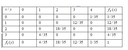
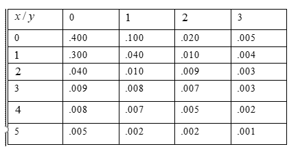
In Given table,X represents the number of syntax errors and Y represents the number of errors in logic.

Problem statement: Determine the probability for selected program have neither of these errors.

Given table

In above table,X represents the number of syntax errors and Y represents the number of errors in logic.

Find the probability

Using given statement to get a required probability such as, p(x = 0,y = 0)

Hence, the value of p(x = 0,y = 0) is 0.4

Hence, the probability that selected program have neither these types of errors as 0.4

Therefore, the probability that selected program have neither these types of errors as 0.4

 

Page 170  Exercise 4  Problem 11

In Given table,X represents the number of syntax errors and Y represents the number of errors in logic.

Problem statement: Determine the probability for selected program at least one syntax error and at most one error in logic.

Given table,In above table,X represents the number of syntax errors and Y

Find the probability

Using given statement to get a required probability such as,

P[X ≥ 1 and Y ≤ 1]

P[X ≥ 1and Y ≤ 1]

[P(X = 1,Y = 0) +  P(X = 2,Y = 0) + P(X = 3,Y = 0)

+ P(X = 4,Y = 0) + P(X = 5,Y = 0) + P(X = 1,Y = 1)

+ P(X = 1,Y = 2) +  P(X = 1,Y = 3) + P(X = 1,Y = 4)

+ P(X = 1,Y = 5)]

P[X ≥ 1and Y ≤ 1]​ = 0.300 + 0.040 + 0.009 + 0.008 + 0.005 + 0.040 + 0.010+ 0.008 + 0.007 + 0.002

P[X ≥ 1and Y ≤ 1] = 0.429

Hence, the probability for selected at least one syntax error and at most one error in logic is 0.429

Therefore, the probability for selected at least one syntax error and at most one error in logic is 0.429

 

Page 170  Exercise 4  Problem 12

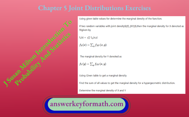
Using given table values for determine the marginal density of the function.

If two random variables with joint density fXY then the marginal density for X denoted as f_x given by

\(f_X(x)=\sum_y f_{X Y}(x, y)\)

 

The mariginal density for y denoted as

\(f_Y(y)=\sum_y f_{X Y}(x, y)\)

 

Given table

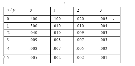
In above table, X represents the number of syntax errors and y represents the number of errors in logic.

Using Given table, sum all values for determine a marginal density

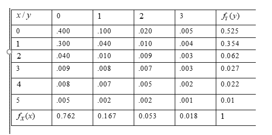
Hence, the marginal density was obtained

Therefore, the marginal density for both values are obtained in above table.

 

Page 170  Exercise 5  Problem 13

On previous example to get a function is, f_xy(x,y)= \(\frac{1.72}{x}\)

If determine a function has to be joint density function satisfies the below condition

\(\int_{-\infty}^{\infty} \int_{-\infty}^{\infty} f_{X Y}(x, y) d x d y=1\)

 

The values of $X$ and $Y$ between 27 ≤ y ≤ x ≤ 33

Given: \(f_{X Y}(x, y)=\frac{1.72}{x}\)

Use continuous joint density function to find the value of P[X ≤ 30 and Y ≤ 28]

P[X ≤ 30 and Y≤ 28]= \(\int_{27}^{30} \int_{27}^{28} f_{X Y}(x, y) d x d y\)

\(=\int_{27}^{30} \int_{27}^{28} \frac{1.72}{x} d x d y\)

 

Integrate depends on y and apply the limit values in given function

\( = 1.72 \int_{27}^{30} \frac{1}{x}[y]_{27}^{28} d x\)

 

\( = 1.72 \int_{27}^{30} \frac{1}{x} d x\)

 

Integrate depends on x and apply the limit values in given function

P[X ≤ 30 and Y≤28] = 1.72× \([\ln x]_{27}^{30}\)

P[X ≤ 30 and Y≤28]  ​= 1.72(3.4012 − 3.2958)

P[X ≤ 30 and Y≤28]  =  0.1813
​
Therefore, using previous example to find a function as f_xy (x,y)= \(\frac{1.72x}{x}\) and the value of P[X ≤ 30 and Y ≤ 28] is 0.1813.

 

Page 170  Exercise 6  Problem 14

On previous example to get a function is,f _xy(x,y) = \(\frac{c}{x}\)

If determine a function has to be joint density function satisfies the below condition \(\int_{-\infty}^{\infty} \int_{-\infty}^{\infty} f_{X Y}(x, y) d x d y\) = 1

The values of X and Y between 27 ≤ y ≤ x ≤ 33

Given: f_xy (x,y) = \(\frac{c}{x}\)

Use continuous joint density function to find the value of c

\(\int_{-\infty}^{\infty} \int_{-\infty}^{\infty} f_{X Y}(x, y) d y d x\) = 1

​\(\int_{27}^{33} \int_{27}^x \frac{c}{x} d y d x\)= 1

Integrate depends on y and apply the limit values in given function

\(\int_{27}^{33}\left(\frac{c}{x} y\right)_{27}^x d x\) = 1

\(\int_{27}^{33}\left(c-\frac{c}{x}(27)\right) d x\) = 1

Integrate depends on x and apply the limit values in given function

\(\int_{27}^{33} c d x-27 \int_{27}^{33} \frac{c}{x} d x\)= 1

6c − 27c (ln(33)−3ln(3)) = 1

6c − 5.4181c = 1

c = \(\frac{1}{0.5819}\)

c  = 1.72
​
Therefore, using previous example to find a function as f XY(x,y) = \(\frac{1.72}{x}\)with 27 ≤ y ≤ x ≤ 33 and the value of c is 1.72

 

Page 170  Exercise 6  Problem 15

On previous example to get a function is \(f_{X Y}(x, y)=\frac{1.72}{x}\)

If determine a function has to be joint density function satisfies the below condition, \(f_X(x)=\int_{-\infty}^{\infty} f_{X Y}(x, y) d y\) 27 ≤ y ≤ x ≤ 33

Given: \(f_{X Y}(x, y)=\frac{1.72}{x}\)

Using given function to get a marginal density

Find the marginal density of X

\(f_X(x)=\int_{-\infty}^{\infty} f_{X Y}(x, y) d y\) \(f_X(x)=\int_{27}^{28} \frac{1.72}{x} d y\)

 

Integrate depends on Y and apply the limit values in given function

\(f_X(x)=1.72\left(\frac{1}{x}\right)[y]_{27}^{28}\)

 

\(f_X(x)=1.72\left(\frac{1}{x}\right)[28-27]\)

 

\(f_X(x)=1.72\left(\frac{1}{x}\right)\)

 

Therefore, Therefore, the marginal density for X and the value of P[X≤28] is \(f_{X Y}(x, y)=\frac{1.72}{x}\)

 

Page 170  Exercise 7  Problem 16

Given problem, f_xy (x,y) = c(4x + 2y + 1)

If determine a function has to be joint density function satisfies the below condition

\(\int_{-\infty}^{\infty} \int_{-\infty}^{\infty} f_{X Y}(x, y) d x d y\) = 1

The values of X and Y between

​0 ≤ x ≤ 40

0 ≤ y ≤ 2
​
Given: f_xy (x,y) = c(4x + 2y + 1)

Use continuous joint density function to find the value of c

\(\int_{-\infty}^{\infty} \int_{-\infty}^{\infty} f_{X Y}(x, y) d x d y\) = 1

 

\(\int_0^{40} \int_0^2 c(4 x+2 y+1) d x d y\) = 1

 

Integrate depends on y and apply the limit values in given function

\(c \int_0^{40}\left(4 x y+2 \frac{y^2}{2}+y\right)_0^2 d x\) = 1

 

\(c \int_0^{40}\left(4 x(2)+(2)^2+2\right) d x=\) 1

 

Integrate depends on x and apply the limit values in given function,

\(c \int_0^{40}(8 x+6) d x\)= 1

\(c\left(\frac{8 x^2}{2}+6 x\right)_0^{40}\)= 1

\(c\left(\frac{8(40)^2}{2}+6(40)\right)\)= 1

6640c  = 1

c = \(\frac{1}{6640}\)

Therefore, the given function fXY (x,y)=c(4x+2y+1) and the value of c is \(\frac{1}{6640}\)= 1

 

Page 170  Exercise 7  Problem 17

To solve this, we need to integrate the PDF where X and Y defined as follow.

​P(x > 20,y ≥ 1)

20 < x ≤ 0,1 ≤ y ≤ 2

P(x > 20,y ≥ 1) = 1 \(\int_1^2 \int_{20}^{40} \frac{1}{6640}(4 x+2 y+1) d x d y\)

P(x > 20,y ≥ 1)  =  \(\frac{1}{6640} \int_1^2\left(\frac{4 x^2}{2}+2 y x+x\right) \int_{20}^{40} d y\)

P(x > 20,y ≥ 1)  = \(\frac{1}{6640} \int_1^2(40 y+2420) d y\)

P(x > 20,y ≥ 1)  = \(\frac{1}{6640} \int_1^2(40 y+2420) d y\)

P(x > 20,y ≥ 1)  = \(=\frac{1}{6640}(2480)\)

P(x > 20,y ≥ 1)  = \(\frac{38}{83}\)

The probability of temperature is P(x > 20,y ≥ 1) =\(\frac{38}{83}\)

 

Page 171  Exercise 8  Problem 18

Note that the integral of a valid joint density is equal to 1.

To verify joint density for a two-dimensional random variable.

f _xy (x,y) =  \([\frac{1}{x}\),o < y < x < 1

That the integral of a valid joint density is equal to 1.

1= \(1\iint_R f_{X, Y}(x, y), o<y<x<1\)

= \(\int_0^1 \int_0^x \frac{1}{x} d y d x\)

= \(\left.\int_0^1\left(\frac{y}{x}\right)\right|_0 ^x d x\)

= \(\left.(x)\right|_0 ^1\)

1 = 1

It is a joint density variable.

 

Page 171   Exercise 8  Problem 19

We can get the probability by integrating it into the following regions.

To find P(X ≤ 0.5 and Y ≤ 0.25)

We can get the probability by integrating it on the following regions

0 < y ≤ 0.25

0.25≤ x < 0.5

Thus, we get that

P(X ≤ 0.5 and Y ≤ 0.25) = \(\int_{0.25}^{0.5} \int_0^{0.25} \frac{1}{x} d y d x\)

P(X ≤ 0.5 and Y ≤ 0.25)  = \(\left.\int_{0.25}^{0.5}\left(\frac{y}{x}\right)\right|_0 ^{0.25} d x\)

P(X ≤ 0.5 and Y ≤ 0.25)  = \(\left.0.25[\ln (x)]\right|_0 ^{0.25}\)

P(X ≤ 0.5 and Y ≤ 0.25)  = 0.25 [(ln(0.5)] − [ln(0.25)]

P(X ≤ 0.5 and Y ≤ 0.25)  = 0.1733

Hence, we have found the answer for P(X ≤ 0.5and Y ≤ 0.25) = 0.1733

 

Page 171  Exercise 9  Problem 20

The marginal density distribution of a subset of a collection of random variables is the probability distribution.

To find the marginal densities for X and Y.

\(f_{X, Y}(x, y) = \frac{x^2 y^2}{16}, 0 \leq x, y \leq 2\)

 

To calculate the marginal density for X, by definition, we have to calculate the integral

\(\left.f_X(x)=\int \mathbb{r} f_{(} X, Y\right)(x, y) d y\)

 

By plugging in the values where y is defined and the expression for joint density function, we obtain.

\(f_X(x)=\int_0^2 \frac{x^3 y^3}{16} d y=\frac{x^3}{64}(16-0)=\frac{x^3}{4}\), 0 ≤ x ≤ 2
​

To calculate the marginal density for Y, by definition, we have to calculate the integral

\(\left.f_Y(y)=\int \mathbb{r} f_{(} X, Y\right)(x, y) d x\)
​

By plugging in the values where y is defined and the expression for joint density function, we obtain.

\(f_X(x)=\int_0^2 \frac{x^3 y^3}{16} d y\)
​
\(=\frac{x^3}{64}(16-0)\)

\(=\frac{x^3}{4}\), 0 ≤ x ≤ 2

\(\frac{x^3}{4}\) 0 ≤ x ≤ 2

\(\frac{x^3}{4}\) 0 ≤ x ≤ 2

⇒ \(f_Y(y)=\frac{y^3}{4}, 0 \leq y \leq 2\)

 

Page 171  Exercise 9  Problem 21

The marginal density distribution of a subset of a collection of a random variables is the probability distribution.

To explain if X and Y are independent?

To check if X and Y are independent, we can simply check whether or not the following equation is fulfilled.

f_x,y(x,y) =  f_x(x) f_y(y)

By substituting the calculated expression , we obtain

\(f_{X, Y}(x, y)=\frac{x^3 y^3}{16}=\frac{x^3}{4} \frac{y^3}{4}=f_X(x) f_Y(y)\)

 

Hence X and Y are indeed independent.

Hence X and Y are indeed independent.

 

Page 171  Exercise 9  Problem 22

The marginal density distribution of a subset of a collection of random variables is the probability distribution.

To find P(X ≤ 1)

To find the probability P(X≤1), by definition, we have to calculate integral

P(X≤1) \(=\int_{-\infty}^1 f_X(x) d x\)

By substituting the given expression for the marginal density function and the values where x is defined, we proceed to calculate

P(X ≤ 1) \(\left.=\int_0^{\frac{x 3}{4}} d x=\frac{1}{16}-(1-0)=\frac{(}{1}\right)(16)\)

Therefore, the joint density for (X,Y) is given by \(\frac{1}{6}\)

 

Page 171  Exercise 10  Problem 23

f_x,y(x,y) = c,   20 < x < y < 40 The integral of the PDF should always be equal to l, where x and y is defined.

Thus we get

\(=\iint_R f_{X, Y}(x, y) d x d y\)

 

\(=\int_{20}^{40} \int_{20}^y c d x d y\)
​
\(=c \int_{20}^{40}(y-20) d y\)

\(=\left.c\left(\frac{y^2}{2}-20 y\right)\right|_{20} ^{40}\)

= c (200)

= c\(\frac{1}{200}\)

The value of c is c\(\frac{1}{200}\)

 

Page 171  Exercise 10  Problem 24

The integral of the PDF should always be equal to l, where x and y are defined, then integrating the PDF.

To find the probability that the carrier will pay at least $25 per barrel and the refinery will pay at most $30 per barrel for the oil.

We can express the problem

P(X ≥ 25 and Y ≥ 30)

By integrating the PDF, we get that
​
​P(X ≥ 25 and Y ≥ 30)

​​P(X ≥ 25 and Y ≥ 30\(=\int_{30}^{40} \int_{25}^y \frac{1}{200} d x d y\)

​P(X ≥ 25 and Y ≥ 30) = \(\frac{1}{200} \int_{30}^{40}(y-25) d y\)

​P(X ≥ 25 and Y ≥ 30)= \(\left.\frac{1}{200}\left(\frac{y^2}{2}-25 y\right)\right|_{30} ^{40}\)

​P(X ≥ 25 and Y ≥ 30)= \(\left.\frac{1}{200}\left(\frac{y^2}{2}-25 y\right)\right|_{30} ^{40}\)

​P(X ≥ 25 and Y ≥ 30)= \(\frac{1}{200}\)

​P(X ≥ 25 and Y ≥ 30)= \(\frac{1}{2}\)

P(X ≥ 25 and Y ≥ 30) = \(\frac{1}{2}\)

 

Page 171  Exercise 10  Problem 25

The integral of the PDF should always be equal to l, where x and y are defined, then integrating the PDF.

To find the probability that the price paid by the refinery exceeds that of the carrier by at least $10 per barrel.

We can express the problem

P(Y > X + 10)

Now if we graph the domain, we get

 

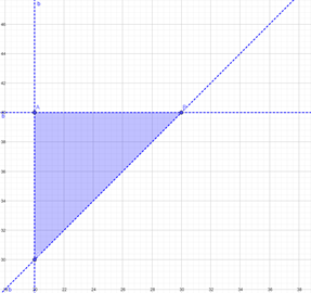
Where

Point A = (20,40)

Point B = (30,40)

Point C = (20,30)

CB  = y − 10

By integrating the PDF
​
​P(Y>X+10)= \(\int_{30}^{40} \int_{25}^y \frac{1}{200} d x d y\)

\(=\left.\frac{1}{200} \int_{30}^{40}(x)\right|_{20} ^{y-10} d y\)

 

\(=\frac{1}{200} \int_{30}^{40}(y-10-20) d y\)

 

\(=\frac{1}{200} \int_{30}^{40}(y-30) d y\)

 

\(=\left.\frac{1}{200}\left(\frac{y^2}{2}-30 y\right)\right|_{30} ^{40}\)

 

= \(\frac{50}{200}\)

 

= 0.25

The probablity is P(Y > X + 10) = 0.25

 

Page 172  Exercise 11 Problem 26

From Continuous Joint density we get that the three properties and identify a function as a density (X₁,X₂,X₃,….. .X_n) f X₁, X₂, X₃ ,. ….. X_n(x₁,x₂,x₃, ….. .x₁ )≥0]−∞<X_i< ∞

For all Xi where i is from 1 to n

\(\int_{-\infty}^{\infty} \int_{-\infty}^{\infty} \int_{-\infty}^{\infty} \cdots \cdots \int_{-\infty}^{\infty}\) f X₁, X₂, X₃ ,…… X₁ (x₁ ,x₂,x₃,……x₁ ) dx₁ dx₂ dx₃……..

P[a ≤ X₁ ≤ b,c ≤ X ≤ d,e ≤ X₃ ≤ f,…..,g ≤ X₁ ≤ h

\(\int_a^b \int_c^d \int_e^f \cdots \cdots \int_g^h\)  f X₁, X₂, X₃ ,…… X(x₁,x₂,x₃,……x_n) dx₁dx₂ dx₃ ………..;. Where a, b, c, …., h are real

Hence, a, b, c, …., h is called the joint density for (X₁ ,X₂,X₃,…..,X_n)