
J.Susan Milton Introduction To Probability And Statistics Principles And Applications Chapter 7 Estimation Descriptive Distributions
Introduction To Probability And Statistics Chapter 7 Exercises Solutions Page 221 Exercise 1 Problem 1
Given problem, X1,X2,X3 ,…..,X20
In the given information, the population mean μ and variance σ were given.
Using the given values to find the sample mean and variance value.
Given: The population mean(μ)is 8 and the variance (σ)is 5.
Determine the mean of \((\bar{X})\)
The sample mean \((\bar{X})\) is an unbiased estimator of the population mean(μ)
The mean \((\bar{X})\) of the sample m X1,X2,X3 ,…..,X20 is the population mean.
Hence, the sample mean value is \((\bar{X})\) = 8
Determine the variance of \((\bar{X})\)
var \((\bar{X})\) = \(\frac{\sigma^2}{n}\)
Substitute n = 20 and σ2 = 5 in previous term
Var \((\bar{X})\) = \(\frac{5}{20}\)= 0.25
Therefore, the mean and variance of \((\bar{X})\) is Mean: 8 Variance: 0.25
Read and Learn More J Susan Milton Introduction To Probability And Statistics Solutions
J.Susan Milton Introduction To Probability And Statistics Principles And Applications Chapter 7 Page 221 Exercise 2 Problem 2
Therefore, an unbiased estimator for the given parameter λs is X. X is the unbiased estimator of λs
J.Susan Milton Introduction To Probability And Statistics Principles And Applications Chapter 7 Page 221 Exercise 3 Problem 3
Given problem statement, X is the number of paint defects in a square yard section of car body painted by robot.
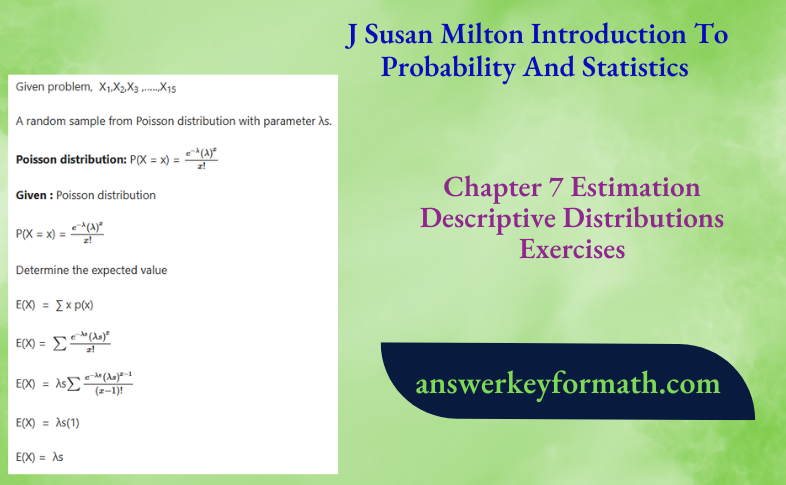
A random sample from Poisson distribution with parameter λs.
Poisson distribution: P(X = x) = \(\frac{e^{-\lambda}(\lambda)^x}{x !}\)
Given : The random variable X is the number of paint defects in a square yard section of car body painted by robot.
Also X is the Poisson distribution with parameter λs.
Find the unbiased estimate for λs
Hence, the sample mean is the unbiased estimator of the population mean.
Then the estimator is
\(\hat{\mu}=\bar{X}\) ,\(\widehat{\lambda s}=\bar{X}\)
Therefore, an unbiased estimator for λs \(\hat{\mu}=\bar{X}\) ,\(\widehat{\lambda s}=\bar{X}\)
J. Susan Milton Estimation Chapter 7 Descriptive Distributions Answers Page 221 Exercise 3 Problem 4
Given problem statement,X is the number of paint defects in a square yard section of car body painted by robot.
A random sample from Poisson distribution with parameter λs.
Determine the unbiased estimate for the average number of flaws per square yard.
Given: The random variable X is the number of paint defects in a square yard section of car body painted by robot.
Also X is the Poisson distribution with parameter λs.
Find the unbiased estimate for λs
Hence, the sample mean is the unbiased estimator of the population mean. Then the estimator is
\(\hat{\mu}=\bar{X}\), \(\widehat{\lambda s}=\bar{X}\)
Determine the unbiased estimate for the average number of flaws per square yard is
ΣiXi = 8 + 0 + 2 + 5 + 3 + 7 + 0 + 1 + 9 + 10 + 12 + 6 = 63
λ8 = \(\frac{63}{12}\)
λ8 = 5.25
Therefore, the unbiased estimate for the average number of flaws per square yard is, 5.25
J.Susan Milton Introduction To Probability And Statistics Principles And Applications Chapter 7 Page 221 Exercise 3 Problem 5
Given problem statement,X is the number of paint defects in a square yard section of car body painted by robot.
A random sample from Poisson distribution with parameter λs.
Determine the unbiased estimate for the average number of flaws per square foot.
Initally,Determine the unbiased estimate for the average number of flaws per square yard is
ΣiXi = 8 + 0 + 2 + 5 + 3 + 7 + 0 + 1 + 9 + 10 + 12 + 6 = 63
λ8 = \(\frac{63}{12}\)
λ8 = 5.25
Determine the unbiased estimate for the average number of flaws per square foot is
One yard = Three feet
Hence, unbiased estimate
5.25 × 3 = 15.75
Therefore, the unbiased estimate for the average number of flaws per square foot is 15.75
Solutions To Estimation And Descriptive Distributions Exercises Chapter 7 Milton Page 221 Exercise 4 Problem 6
Given problem statement,X is the number of requests for the system received per hour.
A random sample from Poisson distribution with parameter λs.
Poisson distribution: P(X = x) = \(\frac{e^{-\lambda}(\lambda)^x}{x !}\)
Given : The random variable X is the number of requests for the system received per hour.
Also X is the Poisson distribution with parameter λs.
Find the unbiased estimate for λs
Hence, the sample mean is the unbiased estimator of the population mean.
Then the estimator is \(\hat{\mu}=\bar{X}\), \(\widehat{\lambda s}=\bar{X}\)
J.Susan Milton Introduction To Probability And Statistics Principles And Applications Chapter 7 Page 221 Exercise 4 Problem 7
Given problem statement,X is the number of requests for the system received per hour.
A random sample from Poisson distribution with parameter λs.
Determine the unbiased estimate for the average number of request received per hour.
Given : The random variable X is the number of requests for the system received per hour.
Also X is the Poisson distribution with parameter λs.
Find the unbiased estimate for λs
Hence, the sample mean is the unbiased estimator of the population mean. Then the estimator is
\(\hat{\mu}=\bar{X}\) , \(\widehat{\lambda s}=\bar{X}\)
Determine the unbiased estimate for the average number of requests received per hour is
ΣiXi = 25 + 30 + 10 + 20 + 24 + 23 + 20 + 15 + 4 = 171
λ8 = \(\frac{171}{9}\)
λ8 = 19
Therefore, the unbiased estimate for the average number of flaws per square yard is 19.
Chapter 7 Estimation And Distributions Examples And Answers Susan Milton Page 221 Exercise 4 Problem 8
Given problem statement,X is the number of requests for the system received per hour.
A random sample from Poisson distribution with parameter λs.
Determine the unbiased estimate for the average number of request received per quarter hour.
Determine the unbiased estimate for the average number of requests received per hour is
ΣiXi = 25 + 30 + 10 + 20 + 24 + 23 + 20 + 15 + 4 = 171
λ8 = \(\frac{171}{9}\)
λ8 = 19
Determine the unbiased estimate for the average number of requests received per quarter hour is
1hour = 60minutes
45 Minutes = \(\frac{45}{60}\) hour
Hence, unbiased estimate is
19 × \(\frac{45}{60}\)
= 14.25
Therefore, the unbiased estimate for the average number of requests received per quarter hour is,14.25
J.Susan Milton Introduction To Probability And Statistics Principles And Applications Chapter 7 Page 222 Exercise 5 Problem 9
Given problem statement,X is the distance in inches from the anchored end of rod to the crack location.
A random sample from binomial distribution with interval (0,b).
Determine the unbiased estimator for the average distance.
Given: The random samples X defines the distance in inches from the anchored end of rod to the crack location.
Also X follows the binomial distribution with interval(0,b).
Hence, the sample mean value is the unbiased estimator for the population mean.
Find the unbiased estimator for the average distance \(\hat{\mu}=\bar{X}\)
Therefore, the unbiased estimator for the average distance in inches from the anchored end of rod to the crack location is \(\hat{\mu}=\bar{X}\)
Probability And Statistics J. Susan Milton Chapter 7 Solved Step-By-Step Page 222 Exercise 5 Problem 10
Given problem statement is the distance in inches from the anchored end of rod to the crack location.
A random sample from binomial distribution with interval (0,b).
Next determine the estimate for p at approximately.
Given: The random samples X defines the distance in inches from the anchored end of rod to the crack location..
Also X follows the binomial distribution with interval (0,b).
Hence, the sample mean value is the unbiased estimator for the population mean.
Find the unbiased estimator for the average distance \(\hat{\mu}=\bar{X}\)
Determine the variance for X is s2
s2 \(=\frac{\sum\left(X_i-\bar{X}\right)^2}{n-1}\)
s2 = \(\frac{1}{10 – 1}\) ((10−9.7)2+(8−9.7)2+(7−9.7)2 + (9−9.7)2 + (11−9.7)2 + (10−9.7)2 + (12−9.7)2 +(9−9.7)2 + (8−9.7)2 +(13−9.7)2)
s2 =\(\frac{0.09+2.89+7.29+0.49+1.69+0.09+5.29+0.49+2.89+10.89}{9}\)
s2 = \(\frac{32.1}{9}\)
s2 = 3.567
Therefore, an estimate for p based on the given data it is approximately 3.567.
J.Susan Milton Introduction To Probability And Statistics Principles And Applications Chapter 7 Page 222 Exercise 5 Problem 11
Given problem statement,X is the distance in inches from the anchored end of rod to the crack location.
A random sample from binomial distribution with interval (0,b).
Next determine the estimate for b.
Given: The random samples X defines the distance in inches from the anchored end of rod to the crack location..
Also X follows the binomial distribution with interval(0,b).
Hence, the sample mean value is the unbiased estimator for the population mean.
Find the unbiased estimator for the average distance \(\hat{\mu}=\bar{X}\)
Equating \(\bar{X}\) and E(x)
\(\frac{b}{2}\) = 9.7
b = 9.7 × 2
b = 19.4
Therefore, an estimate for b based on the given data is 19.4.
Online Help For J. Susan Milton Estimation Chapter 7 Exercises Page 222 Exercise 6 Problem 12
Given problem statement, showS is not unbiased estimator for σ.
Assume that E(S)=σ and using the contradiction method to show that S is not unbiased estimator for σ.
Given: Hence, the sample variance value is the unbiased estimator for the population variance.
Show that S is not unbiased estimator
E(S)= σ2
Assume,E(S) = σ
Based on theorem 3.3.2
V(X) = E(X2) −(E(X))2
Hence
V(S)=E(S2) − (E(S))2
V(S) = σ2 − σ2
V(S) = 0
Therefore,S is not unbiased estimator for σ because the variance value is zero.
J.Susan Milton Introduction To Probability And Statistics Principles And Applications Chapter 7 Page 222 Exercise 7 Problem 13
Given problem statement, k independent random samples and it generates unbiased estimators for the mean value.
Just show that the arithmetic average is an unbiased for μ.
So proof \(E\left(\frac{\bar{X}_1+\bar{X}_2+\ldots+\bar{X}_k}{k}\right)=\mu\)
Given: show that arithmetic average of the estimator is unbiased for μ.
Prove that \(E\left(\frac{\bar{X}_1+\bar{X}_2+\ldots+\bar{X}_k}{k}\right)=\mu\)
Mean value of the estimator is, E[Xi] = μ
\(E\left(\frac{X_1+X_2+\ldots+X_k}{k}\right)=E\left[\frac{1}{k}\left(\bar{X}_1+\bar{X}_2+\ldots+\bar{X}_k\right)\right]\)\(E\left(\frac{\bar{X}_1+\bar{X}_2+\ldots+\bar{X}_k}{k}\right)=\frac{1}{k} E\left[\bar{X}_1+\bar{X}_2+\ldots+\bar{X}_k\right]\)
\(E\left(\frac{\bar{X}_1+\bar{X}_2+\ldots+\bar{X}_k}{k}\right)=\frac{E\left[\bar{X}_1\right]+E\left[\bar{X}_2\right]+\ldots+E\left[\bar{X}_k\right]}{k}\)
\(E\left(\frac{\bar{X}_1+\bar{X}_2+\ldots+\bar{X}_k}{k}\right)=\frac{\mu+\mu+\ldots \mu}{k}\)
\(E\left(\frac{\bar{X}_1+\bar{X}_2+\ldots+\bar{X}_k}{k}\right)=\frac{k \mu}{k}\)
\(E\left(\frac{\bar{X}_1+\bar{X}_2+\ldots+\bar{X}_k}{k}\right)=\mu\)
Therefore, the arithmetic average of the estimator \(E\left(\frac{\bar{X}_1+\bar{X}_2+\ldots+\bar{X}_k}{k}\right)=\mu\) is an unbiased forμ and its proved.
Step-By-Step Guide To Estimation Exercises Chapter 7 Milton Page 222 Exercise 7 Problem 14
iGiven problem:
\(\bar{X}\) = 0.8, n1 = 9
\(\bar{X}\) = 0.95, n2 = 3
\(\bar{X}\) = 0.7, n3 = 200
Using previous value, for determine the averaging of three values to get the unbiased estimator for μ.
On previous lesson, the arithmetic average of the estimator is unbiased for μ.
\(E\left(\frac{\bar{X}_1+\bar{X}_2+\ldots+\bar{X}_k}{k}\right)=\mu\)
Given:
\(\bar{X}\) = 0.8, n1 = 9
\(\bar{X}\) = 0.95, n2 = 3
\(\bar{X}\) = 0.7, n3 = 200
Determine average of three values
\(\widehat{\mu}=\frac{\bar{X}_1+\bar{X}_2+\ldots+\bar{X}_k}{-k}\)
⇒ \(\widehat{\mu}=\frac{\bar{X}_1+\bar{X}_2+\bar{X}_3}{3}\)
⇒ \(\widehat{\mu}=\frac{0.8+0.95+0.7}{3}\)
⇒ \(\widehat{\mu}=\frac{2.45}{3}\)
⇒ \(\widehat{\mu}\) = 0.8167
Therefore, Averaging the three values to get the estimate for μ is 0.8167.
J.Susan Milton Introduction To Probability And Statistics Principles And Applications Chapter 7 Page 222 Exercise 7 Problem 15
Given problem: \(=\frac{n_1 X_1+n_2 X_2+\ldots+n_k X_k}{n_1+n_2+\ldots+n_k}\)
Just show that given is an un biased for μ .so proof, E(\(\widehat{\mu_w}\)) = μ
Given: \(=\frac{n_1 X_1+n_2 X_2+\ldots+n_k X_k}{n_1+n_2+\ldots+n_k}\)
Then prove , E(\(\widehat{\mu_w}\)) = μ

Therefore, given \(\widehat{\mu_w}\) Is ann unbiased estimator for μ and its proved
Exercise Solutions For Chapter 7 Susan Milton Estimation And Distributions Page 222 Exercise 7 Problem 16
Previous problem: \(\widehat{\mu_w}\) = \(=\frac{n_1 X_1+n_2 X_2+\ldots+n_k X_k}{n_1+n_2+\ldots+n_k}\)
Using previous problem data and next deterine the estimate for based on the previous problem.
Given: \(=\frac{n_1 X_1+n_2 X_2+\ldots+n_k X_k}{n_1+n_2+\ldots+n_k}\)
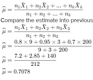
Therefore compared to the previous problem then the weighted average mean is less than mean.
J.Susan Milton Introduction To Probability And Statistics Principles And Applications Chapter 7 Page 223 Exercise 8 Problem 17
Given problem statement,X defines the number of heads obtained when a coin is tossed four times.
Determine the expected value E[X] and variance Var[X] for the variable X.
Given: The random variable X defines the number of heads obtained when a coin is tossed four times.
Also X follows the binomial distribution with parameters
n = 4
p = \(\frac{1}{2}\)
Determine the expected value
E[X] = np
E[X]= 4 × \(\frac{1}{2}\)
E[X] = 2
Find the variance
Var[X] = np(1 − p)
Var[X] = 4 × \(\frac{1}{2}\) (1−\(\frac{1}{2}\))
Var[X]= 4 ×\(\frac{1}{2}\) × \(\frac{1}{2}\)
Var[X] = 1
Therefore, the expected value and variance for the variable X is Expected Value: E[X] = 2, Variance: Var[X] = 1
Page 223 Exercise 8 Problem 18
Given problem statement,X defines the number of heads obtained when a coin is tossed.
The number of heads obtained at 10 times. That means X = 10 and binomial distribution with parameters
n = 4
p = \(\frac{1}{2}\)
Given: The random variableX defines the number of heads obtained when a coin is tossed four times.
Also X follows the binomial distribution with parameters,
n = 4
p = \(\frac{1}{2}\)
When heads obtained at ten times.
That means X = 10 and apply all values in the binomial distribution formula
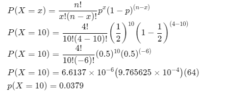
Therefore, the probability for obtain the number of heads at 10 times, 0.0379.
J.Susan Milton Introduction To Probability And Statistics Principles And Applications Chapter 7 Page 223 Exercise 8 Problem 19
Given problem statement,X defines the number of heads obtained when a coin is tossed.
Determine the expected value E[X] and variance Var[X]
for based on 10 observations of the variable X.
Given: The random variable defines the number of heads obtained when a coin tossed.
That means [X = 10] and binomial distribution with parameters
n = 4
p = \(\frac{1}{2}\)
The mean and variance was given
E[X] = 2
Var[X] = 1
Then determine the mean and variance for ten observations.
Mean is summation of all observations divided by number of observations.
The means value is 2.
Variance is sum of squares of each observation subtracted by the mean.
Hence, the variance value is 1
Therefore, based on 10 observations the expected value and variance for the variable X is Expected Value: E[X] = 2 Variance: Var[X] = 1
Page 223 Exercise 8 Problem 20
Given problem statement, X defines the number of heads obtained when a coin is tossed.
The variance Var[X] of the variable X is an unbiased estimate for s2.
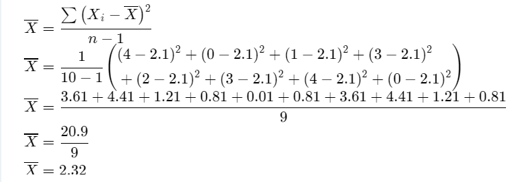
Next determine the variance of the value \(\bar{X}\)
\(\bar{X}=\frac{\sum\left(X_i-\bar{X}\right)^2}{n-1}\)
Given: The random variable defines the number of heads obtained when a coin tossed.
Apply n = 10 for the observations
The unbiased estimate for the variance of X is s2.
Then the \(\bar{X}\)
J.Susan Milton Introduction To Probability And Statistics Principles And Applications Chapter 7 Page 223 Exercise 9 Problem 21
Given: The Random Samples are X1,X2,X3 ,…..,Xn with mean and variance.
Using mean μ and the variance σ2
Value for prove that the below function
\(\frac{\sum\left(X_i-\bar{X}\right)^2}{n}=\frac{(n-1) s^2}{n}\)
Given: The Random Samples are X1,X2,X3 ,…..,Xn with mean μ and variance σ2.
Prove that \(\frac{\sum\left(X_i-\bar{X}\right)^2}{n}=\frac{(n-1) s^2}{n}\) and E(s2 ) = σ2
Consider LHS
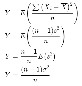
Therefore, the Random Samples X1,X2,X3 ,…..,Xn with mean μ Value and variance σ2 Value for \(\frac{\sum\left(X_i-\bar{X}\right)^2}{n}=\frac{(n-1) s^2}{n}\) and its proved
Page 223 Exercise 10 Problem 22
Given: The Random Sample X1,X2,X3 ,…..,Xm with size m and parameter n.
Using method of moments technique to Determine the first moment of the given sample.
Given: The Random Sample X1,X2,X3 ,…..,Xm with size m and parameter n.
Also, it follows the Binomial Distribution X1,X2,X3 ,…..,Xm
Use method of moments to find the estimator for p,
M1 = \(\frac{\sum_i X_i}{m}=\bar{X}\)
Find the first moment of the sample, E(X) = np
\(n \hat{p}=\bar{X}\) \(\hat{p}=\frac{\bar{X}}{n}\)
Therefore, using Method of Moments technique for find the estimator of p is \(\hat{p}=\frac{\bar{X}}{n}\) and its proved.