
J.Susan Milton Introduction To Probability And Statistics Principles And Applications Chapter 8 Inferences On The Mean And Variance Of A Distribution
Introduction To Probability And Statistics Chapter 8 Exercises Solutions Page 263 Exercise 1 Problem 1
Given problem statement, when programming from a terminal, one random variable response time was recorded in seconds.
These data are tabled also a table was given.
Next draw the stem and leaf diagram and assume the normality is reasonable or not
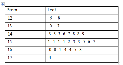
Stem and leaf plot response time N = 30
Leaf unit = 0.010
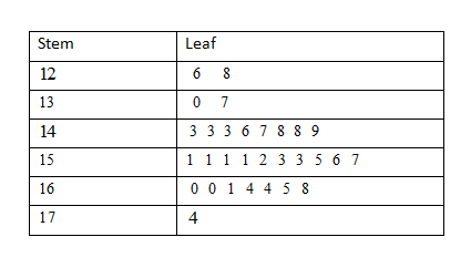
Therefore, the step plot shows the data is equally distributed on both sides. So, the assumptions of normality appear reasonable.
Read and Learn More J Susan Milton Introduction To Probability And Statistics Solutions
J.Susan Milton Introduction To Probability And Statistics Principles And Applications Chapter 8 Page 263 Exercise 1 Problem 2

Given: When programming from a terminal, one random variable response time was recorded in seconds.
These scenarios can be represented in X.
n = 30
Determine the \(\bar{X}\) value
\(\overline{X_n}=\frac{\sum X_i}{n}\)
\(\bar{X}\)n = \(\left(\begin{array}{l}
1.48+1.26+1.52+1.56+1.48+1.46+1.30+1.28+ \\
1.43+1.43+1.55+1.57+1.51+1.53+1.68+1.37+ \\
1.47+1.61+1.49+1.43+1.64+1.51+1.60+1.65+ \\
1.60+1.64+1.51+1.51+1.53+1.74
\end{array} 30\right.\)
Therefore, an unbiased point estimate for σ2 is 0.0129
J.Susan Milton Introduction To Probability And Statistics Principles And Applications Chapter 8 Page 263 Exercise 1 Problem 3
From previous problem the point estimate of σ2 is s2 was obtained and using this value to find a 95 confidence interval for σ2
First determine the value of α
α = 1 − confidence level
Given :
From previous problem the point estimate of σ2 is s2 = 0.0129
Find the value of α is
α = 1 − 95
α = 0.05
n = 30
Find a 95 confidence interval for σ2
Formula is , L1 ≤ σ2 L2
\(\frac{(n-1) S^2}{\chi_{\frac{\alpha}{2}}^2} \leq \sigma^2 \leq \frac{(n-1) S^2}{\chi_{1-\frac{\alpha}{2}}^2}\)
Using chi-square distribution table to find a probability value with corresponds to degrees of freedom.
Probability value0.025 that corresponds to 29 degrees of freedom is 45.7
Probability value 0.0975 that corresponds to 29 degrees of freedom is 16
Determine the confidence interval for σ2
\(\frac{(30-1)(0.0129)}{45.7} \leq \sigma^2 \leq \frac{(30-1)(0.0129)}{16.0}\) \(\frac{0.3741}{45.7} \leq \sigma^2 \leq \frac{0.3741}{16.0}\)
0.00082 ≤ σ2 0.0234
Hence, 95 confidence interval for σ2 is (0.0082,0.0234)
Therefore,95 confidence interval for σ2 is (0.0082,0.0234)
J.Susan Milton Introduction To Probability And Statistics Principles And Applications Chapter 8 Page 263 Exercise 1 Problem 4
From previous problem the point estimate for σ2
Was obtained and using this value to find a 95 confidence interval for σ
First determine the value of α
α = 1 − confidence level
Given :
From previous problem the point estimate for σ2 is 0.0129
Find the value of α is α = 1−95
α = 0.05
n = 30
Find a 95 confidence interval for σ formula is
\(\sqrt{L_1} \leq \sigma \leq \sqrt{L_2}\)\(\sqrt{\frac{(n-1) S^2}{\chi_{\frac{\alpha}{2}}^2}} \leq \sigma \leq \sqrt{\frac{(n-1) S^2}{\chi_{1-\frac{\alpha}{2}}^2}}\)
Using chi-square distribution table to find a probability value with corresponds to degrees of freedom.
Probability value0.95 that corresponds to 29 ,degrees of freedom is 45.7
Probability value 0.025 that corresponds to 29 degrees of freedom is 16
Determine the confidence interval for σ
\(\sqrt{\frac{(30-1)(0.0129)}{45.7}} \leq \sigma \leq \sqrt{\frac{(30-1)(0.0129)}{16.0}}\)
\(\sqrt{0.0082} \leq \sigma \leq \sqrt{0.0234}\)
0.091 0.091 ≤ σ ≤0.153
Hence, 95 confidence interval for σ is (0.091,0.153)
Therefore, 95 confidence interval for σ is (0.091,0.153)
J.Susan Milton Introduction To Probability And Statistics Principles And Applications Chapter 8 Page 263 Exercise 2 Problem 5
Given problem statement, highway engineers have found a sign at night and it depends on its surround luminance.
These scenarios can be represented in X.
These surround luminance data are tabled also a table was given.
Estimate the value of X
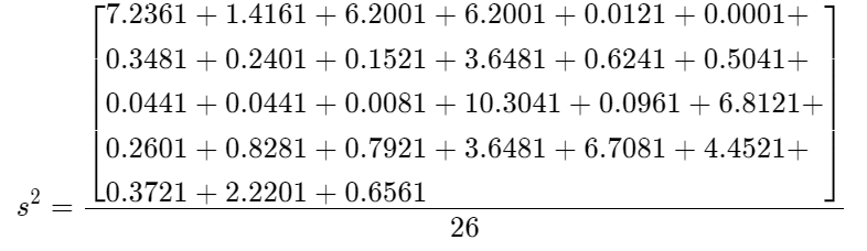
For determine an unbiased estimate for σ2
Formula for find the point estimate of σ2 is s2
s2 \(=\frac{\sum\left(X_i-\bar{X}\right)^2}{n-1}\)
Given : Highway engineers have found a sign at night and it depends on its surround luminance.
These scenario can be represented in X.
n = 30
Determine the \(\bar{X}\) value
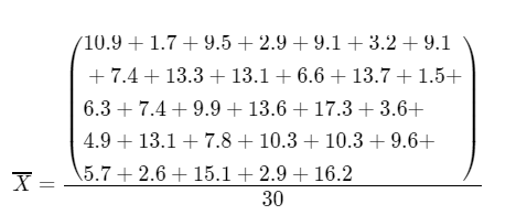
\(\bar{X}\) = \(\frac{258.6}{30}\)
\(\bar{X}\) = 8.62
The point estimate for σ2 is
\(s^2=\frac{\sum\left(X_i-\bar{X}\right)^2}{n-1}\)
s2 = \(
\frac{\sum\left(X_i-\bar{X}\right)^2}{n-1}\)
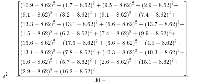
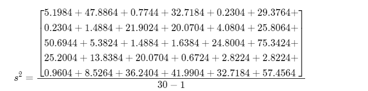
s2 = \(\frac{592.428}{29}\)
s2 = 20.428
Therefore, an unbiased point estimate for σ2 is, 20.428
J.Susan Milton Introduction To Probability And Statistics Principles And Applications Chapter 8 Page 263 Exercise 2 Problem 6
From the previous problem the point estimate for σ2
was obtained and using this value to find a 90 confidence interval for σ.
First determine the value of α, α = 1− confidence level
Given :
From previous probelm the point estimate for σ2 is
20.428
Find the value of α is
α = 1 − 90
α = 0.10
n = 30
Find a 90 confidence interval for σ2
Formula is
L1 ≤ σ2 ≤ L2
\(\frac{(n-1) S^2}{\chi_{\frac{a}{2}}^2} \leq \sigma^2 \leq \frac{(n-1) S^2}{\chi_{1-\frac{a}{2}}^2}\)
Using chi-square distribution table to find a probability value with corresponds to degrees of freedom.
Probability value 0.05 that corresponds to 29 degrees of freedom is 42.557
Probability value 0.95 that corresponds to 29 degrees of freedom is 17.7084
Determine the confidence interval for σ2
\(\frac{(30-1)(20.428)}{42.557} \leq \sigma^2 \leq \frac{(30-1)(20.428)}{17.7084}\)
\(\frac{5924.12}{42.557} \leq \sigma^2 \leq \frac{5924.12}{17.7084}\)
13.9204 ≤ σ2 ≤ 33.4537
Hence, 90 confidence interval for σ2 is (13.9204,33.4537)
Determine the confidence interval for σ
\(\sqrt{L_1} \leq \sigma \leq \sqrt{L_2}\) \(\sqrt{\frac{(n-1) S^2}{\chi_{\frac{a}{2}}^2}} \leq \sigma \leq \sqrt{\frac{(n-1) S^2}{\chi_{1-\frac{\alpha}{2}}^2}}\)\(\sqrt{13.9204} \leq \sigma \leq \sqrt{33.4537}\)
3.731 ≤ σ2 ≤ 5.784
Hence, 90 confidence interval for σ is (3.731,5.784)
Therefore, 90 confidence interval for σ is (3.731,5.784)
J.Susan Milton Introduction To Probability And Statistics Principles And Applications Chapter 8 Page 264 Exercise 3 Problem 7
Given problem statement, Two voltage technique is used to analyze the crystals. Using electron microprobe to measure both quantitative and qualitative measurements.
These data are tabled also a table was given.
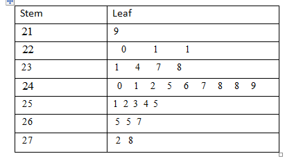
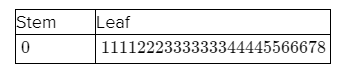
Next draw the stem and leaf diagram and assume the normality is reasonable or not.
Given :
Stem and leaf plot measurement N = 27
The values have been multiplied by 100
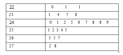
Therefore, the step plot shows the data is equally distributed on both sides. So, the assumptions of normality appear reasonable.
J.Susan Milton Introduction To Probability And Statistics Principles And Applications Chapter 8 Page 264 Exercise 3 Problem 8
Given problem statement, two voltage technique is used to analyze the crystals.
Using electron microprobe to measure both quantitative and qualitative measurements. These scenarios can be represented in X.
These data are tabled also a table was given.
Estimate the value of \(\bar{X}\) for determine an unbiased estimate for σ2
Formula for find the point estimate for σ2 is
\(s^2=\frac{\sum\left(X_i-\bar{X}\right)^2}{n-1}\)
Given: Two voltage technique is used to analyze the crystals. Using electron microprobe to measure both quantiative and qualiitiative measurements.
These scenario can be represented in X.
n = 27
Determine the \(\bar{X}\) value
\(\bar{X}\) = \(\frac{\sum X_i}{n}\)
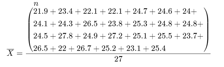
\(\bar{X}\) = \(\frac{663.9}{27}\)
\(\bar{X}\) = 24.59
The point estimate for σ2 is
\(s^2=\frac{\sum\left(X_i-\bar{X}\right)^2}{n-1}\)
s2 = \(\frac{63.8267}{26}\)
s2 = 2.455
Therefore, an unbiased point estimate for σ2 is, 2.455
J.Susan Milton Introduction To Probability And Statistics Principles And Applications Chapter 8 Page 264 Exercise 4 Problem 9
Given problem statement, find the one-sided confidence interval for the upper bound.
Also, an interval in the form of [0,L].
Finally prove that the upper bound confidence interval
L = \(\frac{(n-1) s^2}{\chi_{1-\alpha}^2}\)
Given:
Find an interval in the form of P[σ2 ≤ L] = 1 − α
That means Confidence level = 1 − α
Form the diagram, the evidence is
Determine the confidence interval for σ2
P \(\left(\chi_{1-\alpha}^2 \leq \frac{(n-1) s^2}{\sigma^2}\right)\) = 1 − α
P \(\left(\sigma^2 \leq \frac{(n-1) s^2}{\chi_{1-\alpha}^2}\right)\) = 1 − α
Hence \(=\frac{(n-1) s^2}{\chi_{1-\alpha}^2}\)
Therefore, the confidence interval for upper bound is \(=\frac{(n-1) s^2}{\chi_{1-\alpha}^2}\) and its proved.
J.Susan Milton Introduction To Probability And Statistics Principles And Applications Chapter 8 Page 265 Exercise 5 Problem 10
Given problem statement, Robotic technology was explained.
The Robots are used to apply adhesive to a specified location.
These location data are tabled also a table was given.
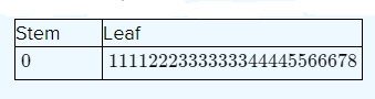
Next draw the stem and leaf diagram and assume the normality is reasonable or not.
Given :
Stem and leaf plot measurement N = 25
The values have been multiplied by 1000
Therefore, the step plot shows the data is equally distributed on both sides. So, the assumptions of normality appear reasonable.
J.Susan Milton Introduction To Probability And Statistics Principles And Applications Chapter 8 Page 265 Exercise 5 Problem 11
Given problem statement, Robotic technology was explained.
The Robots are used to apply adhesive to a specified location. These scenarios can be represented in X.
These location data are tabled also a table was given.
Estimate the value of \(\bar{X}\) For determine an unbiased estimate for σ2
Formula for find the point estimate for σ2 is
\(s^2=\frac{\sum\left(X_i-\bar{X}\right)^2}{n-1}\)
Given : Robotic technology was explained.
The Robots are used to apply adhesive to a specified location.
These scenarios can be represented in X
n = 27
Determine the \(\bar{X}\) value
\(\bar{X}\) = \(\frac{\sum X_i}{n}\)
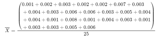
\(\bar{X}\) =\(\frac{0.09}{25}\)
\(\bar{X}\) = 0.0036
The point estimate for σ2 is
\(\frac{\sum\left(X_i-\bar{X}\right)^2}{n-1}\)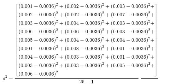
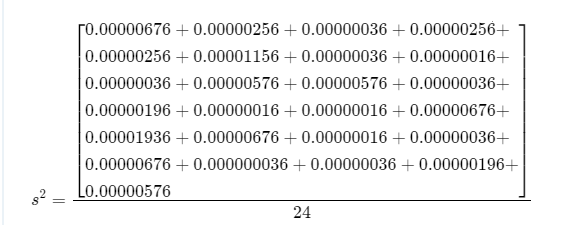
s2 = \(\frac{0.00009}{24}\)
s2 = 0.00000375
Therefore, an unbiased point estimate for σ2 is, 0.00000375
J.Susan Milton Introduction To Probability And Statistics Principles And Applications Chapter 8 Page 265 Exercise 6 Problem 12
Initially understand the theorems and using the theorem to prove that mean and variance values such as E[S2 ]= σ2 and Var S2
= \(\frac{2 \sigma^4}{(n-1)}\)
Show that X be a random variable. The mean and variance is
E[S2 ]= σ2
Var S2 = \(\frac{2 \sigma^4}{(n-1)}\)
From S2 is an unbiased estimator for σ2. Hence? E[S2] = σ2
From using of formula \(\frac{(n-1) S^2}{\sigma^2} \sim \chi_{(n-1)}\)
The variance of the chi squared distribution is n 2(n−1)
Now
Var [ \(\frac{(n-1) S^2}{\sigma^2}\)] = 2(n – 1)
\(\frac{(n-1)^2}{\sigma^4}\)Var S2 = 2(n – 1)
Var S2 = 2(n – 1)\(\frac{\sigma^4}{(n-1)^2}\)
Var s2 =\(\frac{2 \sigma^4}{(n-1)}\)
Therefore, X be a random variable then the mean and variance E[S2 ]= σ2,Var S2 \(\frac{2 \sigma^4}{(n-1)}\) and its proved.
J.Susan Milton Introduction To Probability And Statistics Principles And Applications Chapter 8 Page 265 Exercise 7 Problem 13
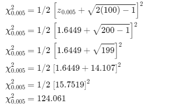
Given Samples: χ0.005 and χ0.95
Formula for find chi squared points: \(\chi_r{ }^2=1 / 2\left[z_r+\sqrt{2 \gamma-1}\right]^2\)
Using above formula to determine the approximate points of the given samples.
Given : χ0.005 and χ0.95
Formula for approximate the chi squared points \(\chi_r{ }^2=1 / 2\left[z_r+\sqrt{2 \gamma-1}\right]^2\)
r is significance level and γ is the degrees of freedom
Approximate the points for χ0.005
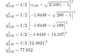
Approximate the points for χ0.95
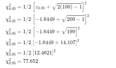
Therefore, approximated points of χ0.005 and χ0.95 is 124.061 and 77.652
J.Susan Milton Introduction To Probability And Statistics Principles And Applications Chapter 8 Page 265 Exercise 7 Problem 14
Given: Standard deviation value is s = 7.5 and sample size is n = 150
Using above values to find the confidence interval on deviation.
Formula for find the confidence interval for deviation
\(\sqrt{L_1}=\sqrt{\frac{(n-1) S^2}{\chi_{\alpha / 2}^2}}\sqrt{L_2}=\sqrt{\frac{(n-1) S^2}{\chi_{1-\alpha / 2}^2}}\)Given: Standard deviation and sample sizes are included below
s = 7.5
n = 150
Formula for find interval
\(\sqrt{L_1}=\sqrt{\frac{(n-1) S^2}{\chi_{\alpha / 2}^2}} \sqrt{L_2}=\sqrt{\frac{(n-1) S^2}{\chi_{1-\alpha / 2}^2}}\)
Determine the interval for χ0.025
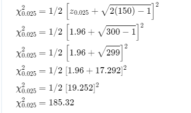
Determine the interval for χ0.025

Confidence interval is
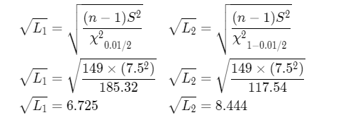
Hence, 95 % confidence interval on the standard deviation is (6.725,8.444)
Therefore,95 % the confidence interval on the standard deviation is(6.725,8.444)
J.Susan Milton Introduction To Probability And Statistics Principles And Applications Chapter 8 Page 266 Exercise 8 Problem 15
Given: Standard deviation value is s = 0.01 and sample size is n = 100
Using above values to find the confidence interval for deviation One sided confidence interval
\(L=\frac{(n-1) s^2}{\chi_{1-\alpha}^2}\)
Given : Standard deviation and sample size is
s = 0.01
n = 100
Formula for find interval
\(L=\frac{(n-1) s^2}{\chi_{1-\alpha}^2}\)
Chi squared points can be approximated by the formula
\(\chi_{1-r}^2=1 / 2\left[z_{1-r}+\sqrt{2 \gamma-1}\right]^2\)
Approximate the points for χ0.95
Determine the confidence interval
\(L=\frac{(n-1) s^2}{\chi_{1-\alpha}^2}\)\(\sqrt{L}=\sqrt{\frac{99 \times(0.01)^2}{77.652}}\)
= 0.0113
Hence, 95 % confidence interval on the standard deviation is (0,0.0113)
Therefore, 95 % confidence interval on the standard deviation is (0,0.0113)
J.Susan Milton Introduction To Probability And Statistics Principles And Applications Chapter 8 Page 266 Exercise 9 Problem 16
Given: t.05 (γ = 8)
In T Distribution table, the cumulative probability values are given.
If find a critical value, look up the confidence interval in the bottom row of the table.
From T distribution table the row locates 8 and the column of P[Tr ≤ t] locate 0.95 which corresponds to the critical value is 1.8595
Hence, the value of t.05 (γ = 8) is 1.8595
Therefore, the value of t.05(γ = 8) is 1.8595
J. Susan Milton Chapter 8 Inferences On Mean And Variance Answers Page 266 Exercise 9 Problem 17
Given: t.95 (γ = 8)
In T Distribution table, the cumulative probability values are given.
If find a critical value, look up the confidence interval in the bottom row of the table.
From T distribution table the row locates 8 and the column of P[Tr ≤ t] locate 0.95 which corresponds to the critical value is −1.8595
Therefore, the value of t.95 (γ = 8) is−1.8595
J.Susan Milton Introduction To Probability And Statistics Principles And Applications Chapter 8 Page 266 Exercise 9 Problem 18
Given: t 0.975 (γ = 12)
In T Distribution table, the cumulative probability values are given.
If find a critical value, look up the confidence interval in the bottom row of the table.
From T distribution table the row locates 12 and the column of P[Tr ≤ t] locate 0.975 which corresponds to the critical value is −2.1788
Hence, the value of t.975 (γ = 12) is −2.1788
Therefore, the value of t 975 (γ = 12) is −2.1788
Solutions To Inferences On Mean And Variance Exercises Chapter 8 Susan Milton Page 265 Exercise 10 Problem 19
In this given question, t value is .05.
In this given question, γ value is 50
Have to find a probability for given t value with given γ value.
Point degree of freedom and search for a given t value.
Given t value = .05.
γ = 50.
By using the t table, t⋅05 (γ = 50) = 1.6759
Hence, the probability of given t value ⋅05 with degree of freedom γ = 50 is 1.6759.
J.Susan Milton Introduction To Probability And Statistics Principles And Applications Chapter 8 Page 265 Exercise 10 Problem 20
In this given question, t value is .025.
In this given question, y value is 75.
Have to find a probability for given t value with given γ value.
Point degree of freedom and search for a given t value.
Given t
value t = .025
γ = 75
By using the t table, t = .025
(γ = 75) = 1.9921
Hence, the probability of given t value .025 with degree of freedom γ = 75 is 1.9921
Chapter 8 Inferences on Mean and Variance examples and answers Susan Milton Page 265 Exercise 10 Problem 21
In this given question, t value is 0.1.
In this given question, γ value is 200.
Have to find a probability for given t value with given γ value.
Point degree of freedom and search for a given t value.
Given
t value = 0.1
γ = 200
By using the t table
t 0⋅1 (γ = 200) = 1.2858
Hence, the probability of given t value 0.1 with degree of freedom γ = 200 is 1.2858
J.Susan Milton Introduction To Probability And Statistics Principles And Applications Chapter 8 Page 266 Exercise 11 Problem 22
In this question, the given data is \(\sum_{i=1}^{20} x_i\) = 25.792 and
\(\sum_{i=1}^{20} x_i^2\) = 33. 261596
Have to find \(\bar{X}\) , s2 , s
\(\bar{X}\) = \(\frac{\sum x_i}{n}\)
s2 = \(\frac{1}{n-1}\left(\sum x_i^2-n(\bar{X})^2\right)\)
s = \(\sqrt{s^2}\)
Given
\(\sum_1^{15} x_i\) = 0.07
\(\sum_1^{15} x_i^2\) = 0.0489
n = 15
\(\bar{X}\) = \(\frac{\sum x_i}{n}\)
\(\bar{X}\) = \(\frac{0.07}{15}\)
\(\bar{X}\) = 0.00467
\(\frac{1}{n-1}\left(\sum x_i^2-n(\bar{X})^2\right)\)
= \(\frac{1}{15-1}\left(0 \cdot 0489-15(0 \cdot 00467)^2\right)\)
= \(\frac{1}{14}(0 \cdot 0489-0 \cdot 000327)\)
= \(\frac{0.048573}{14}\)
= 0.0034695
s = \(\sqrt{s^2}\) = \(\sqrt{0.0034695}\)
s = 0.0589
Hence, the Value of \(\bar{X}\),s 2, s are 0⋅00467, 0⋅0034695,0⋅0589 respectively.
J.Susan Milton Introduction To Probability And Statistics Principles And Applications Chapter 8 Page 266 Exercise 11 Problem 23
To find 95 % confidence interval 100(1 − α)
\(\bar{X} \pm t_{\frac{\alpha}{2}, \frac{n-1 s}{\sqrt{n}}}\) = 0.00467 \(\pm t_{0.05, \frac{15-10.0589}{\sqrt{5}}}\)
= 0⋅00467 ± 1.7693 × 0.0152
= 0.00467 ± 0.0269
= (0⋅00467 − 0.0269, 0.00467 + 0.0269)
= (−0.02223, 0.03157)
Hence,95 % confidence interval on the mean outside diameter of the pipes is(−0.02223,0.03157)
J.Susan Milton Introduction To Probability And Statistics Principles And Applications Chapter 8 Page 266 Exercise 11 Problem 24
The makers of this pipe claim that the mean outside diameter is 1.29, so an average overestimate is 0.05.
The average overestimates the distance by 0.05 which is not reasonable.
Because the overestimates do not lie within 90 confidence interval.
Hence, the confident interval does not lead to suspect this responded.