Probability and Statistics for Engineering and the Sciences 8th Edition Chapter 1 Overview and Descriptive Statistics
Page 24 Problem 1 Answer
Given,To make the Steam-and-Leaf Display:
We select the leading digits, then the digits that come after the leading digits are the leaves.
Then we list the parent values that we have received in a column.
Then we comment on the leaf for all data values associated with the respective parent value.
Then we write down the units of the stem and leaves.
The data given to us in tabular form is:
| 5.9 | 7.2 |
| 7.3 | 6.3 |
| 8.1 | 6.8 |
| 7 | 7.6 |
| 6.8 | 6.5 |
| 7 | 6.3 |
| 7.9 | 9 |
| 8.2 | 8.7 |
| 7.8 | 9.7 |
| 7.4 | 7.7 |
| 9.7 | 7.8 |
| 7.7 | 11.6 |
| 11.3 | 11.8 |
| 10.7 |
If we follow our explanation above, we first obtain the leading digits. These leading digits are:5,6,7,8,9,10,11
Listing the leading digits:
| Stem |
| 5 |
| 6 |
| 7 |
| 8 |
| 9 |
| 10 |
| 11 |
Recording the leaves for each and every observation and obtain the Stem-and-leaf display:
| Stem | Leaf |
| 5 | 9 |
| 6 | 33588 |
| 7 | 234677889 |
| 8 | 127 |
| 9 | 77 |
| 10 | 7 |
| 11 | 368 |
| Stem: ones | Leaf: tenths |
Since the representative strength value is the value that is in the middle, in this case, it would be 7.7.
The observations are also spread out and the values around our representative strength value aren’t symmetrically spread around the middle.
Therefore, the Stem-and-Leaf display is obtained as Stem
The representative strength value is 7.7 and the observations are spread out.
Page 24 Problem 2 Answer
To get the representative value of the force, we will first write down all the values on a screen of the root leaf.
The representative force value is the value in the middle of the root leaf lattice. If the data is symmetrical about the value of the representative force, then the data is said to be undistorted.
The stem-and-leaf display of the values is given as:
| Stem | Leaf |
| 5 | 9 |
| 6 | 33588 |
| 7 | 234677889 |
| 8 | 127 |
| 9 | 77 |
| 10 | 7 |
| 11 | 368 |
| Stem: ones | Leaf: tenths |
The representative strength value for the data is the value in the middle which is 7.7.
The observations are spread out and not symmetric about the representative strength value rather they are more positively skewed.
Hence,the data is not symmetrical and the values aren’t symmetrically distributed around the representative strength value.
It makes sense that the dataset is skewed positively.
Page 24 Problem 3 Answer
Given, In order to obtain the values that lie outside, we’ll first note down all the observations in a stem-and-leaf display.
If some of the values in the data are abnormally deviating, then they are said to be outliers.
The stem-and-leaf display of the values is given as:
| Stem | Leaf |
| 5 | 9 |
| 6 | 33588 |
| 7 | 234677889 |
| 8 | 127 |
| 9 | 77 |
| 10 | 7 |
| 11 | 368 |
| Stem: ones | Leaf: tenths |
We notice that 5.9 and 11.8 differ the most from the rest of the values but not abnormally.
Therefore we can’t say that they are outliers.
Hence,we notice that 5.9 and 11.8 differ the most from the rest of the values but not abnormally.
Therefore we can’t say that they are outliers there are no outliers in the dataset.
Probability And Statistics For Engineering 8th Edition Solutions Exercise 1.2 Page 24 Problem 4 Answer
Given,In order to calculate the proportion of strength observations in this sample exceed 10 MP a, we have to calculate the total number of observed values.
After that we will determine the number of observations that are greater than 10 MP a.
We consider taking the ratio of the both in which the number of observations which are greater than 10 MP a is the numerator and total number of observations is the denominator.
The total number of observations: n=27
Number of observations that are greater than10
MP a:10.7,11.3,11.6,11.8 x=4
The proportion of strength observations in this sample exceed 10 MP a:X/n=4/27
⇒0.1481
Converting the proportion into percentages we get: 14.81%≈15%
Therefore, the proportion of strength observations in this sample which exceed 10 MPa: 15%
Page 24 Problem 5 Answer
Given, To make the Steam-and-Leaf Display:
| Stem (tenths) |
| 0.3 |
| 0.4 |
| 0.5 |
| 0.6 |
| 0.7 |
We choose the leading digits, following that, the digits coming after the leading digits are the leaves.
Then list the values of the stem were obtained in a column.
Note down the leaf for all data values pertaining with the particular stem value.
We then note down the units of the stem and leaves.
The leading digits (tenths) for the dataset are:0.3,0.4,0.5,0.6,0.7
Listing the leading digits:
| Stem | Leaf |
| 0.3 | 156678 |
| 0.4 | 1122222345667880 |
| 0.5 | 14458 |
| 0.6 | 26678 |
| 0.7 | 5 |
| Steam: tenths | Leaf: hundredths |
Recording the leaves for each and every observation and obtain the Stem-and-leaf display:
| Stem | Leaf |
| 0.3 | 156678 |
| 0.4 | 1.12222E+15 |
| 0.5 | 14458 |
| 0.6 | 26678 |
| 0.7 | 5 |
| Steam: tenths | Leaf: hundredths |
We see that the dataset is positively skewed with a representative value of 0.445
Therefore,the dataset following batch of exam scores is positively skewed, uni-modal with a representative value of 0.445.
Page 25 Problem 6 Answer
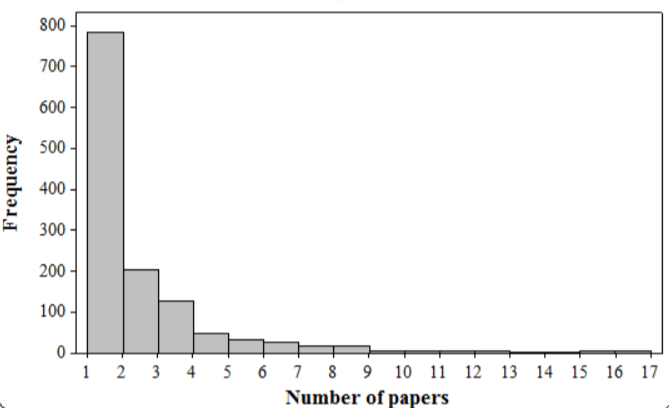
Given, In a study of author productivity a large number of authors were classified according to the number of articles they had published during a certain period.
The results were presented in the given frequency distribution.
We need to construct a histogram corresponding to this frequency distribution.
Also write the most interesting feature of the shape of the distribution.

Now,Based on the given frequency distribution the histogram is plotted as by taking number of papers on horizontal line.
Height of the rectangle bar represents the frequency.
From observing the above plot,the histogram is completely skewed to the right.
Hence,the histogram is highly positive skewed.
Therefore,by using the frequency distribution the histogram plotted can be as follows:
Page 25 Problem 7 Answer
Given,In a study of author productivity a large number of authors were classified according to the number of articles they had published during a certain period.
The results were presented in the given frequency distribution.
We need to find the proportion of these authors published at least five papers.
Also find the proportion for at least ten papers and proportion for more than ten papers.
Now, To find the proportion of these authors published at least five papers:
P(X≥5)=1−P(X<5)
P(X≥5) =1−{P(X=1)+P(X=2)+P(X=3)+P(X=4)}
P(X≥5) =1−{784/1309+204/1309+127/1309+50/1309}
P(X≥5) =1−1165/1309
P(X≥5) =144/1309
P(X≥5) =0.11
Similarly, for the proportion for at least ten papers:
P(X≥10)=39/1309
P(X≥10) ≈0.03
Then,the proportion for more than ten papers:
P(X>10)=32/1309
P(X>10) ≈0.024
Therefore,the proportion of these authors published at least five papers is obtained as 11%.
Similarly,for the proportion of these authors published for at least ten papers is obtained as 3%.
The proportion of these authors published for more than ten papers is obtained as 2.4%.
Chapter 1 Exercise 1.2 Overview And Descriptive Statistics Solved Examples Page 25 Problem 8 Answer
Given, In a study of author productivity a large number of authors were classified according to the number of articles they had published during a certain period.
The results were presented in the given frequency distribution.
Suppose the five 15s, three 16s, and three 17s had been lumped into a single category displayed as≥15.
We need to verify that whether we can draw a histogram with the given data with explanation.
Now, Suppose the five 15s, three 16s, and three 17s had been lumped into a single category displayed as ≥15.
As we can observe that the class is≥15 has no upper bound.
Hence, we are unable to draw a histogram because of the class≥15 with no upper bound specified.
So,from the given data of class which is greater than 15 with no upper bound specified then we are unable to draw a histogram
Page 25 Problem 9 Answer
Given,In a study of author productivity a large number of authors were classified according to the number of articles they had published during a certain period.
The results were presented in the given frequency distribution.
Suppose that instead of the values15,16 and 17 being listed separately, they had been combined into a 15−17 category with frequency 11.
We need to explain whether we able to draw a histogram or not with proper explanation
Now,Combined class of15−17 category with frequency 11.
Width of the class is 2.
So,the area of 11 of the bar equals to product of height and width.
Hence,we can draw histogram with the given data.
Therefore,instead of the values 15,16 and 17 being listed separately, they had been combined into a 15−17 category with frequency 11 then we can draw
histogram with width of class 2 and are a11 of the bar equals to product of height and width.
Page 25 Problem 10 Answer
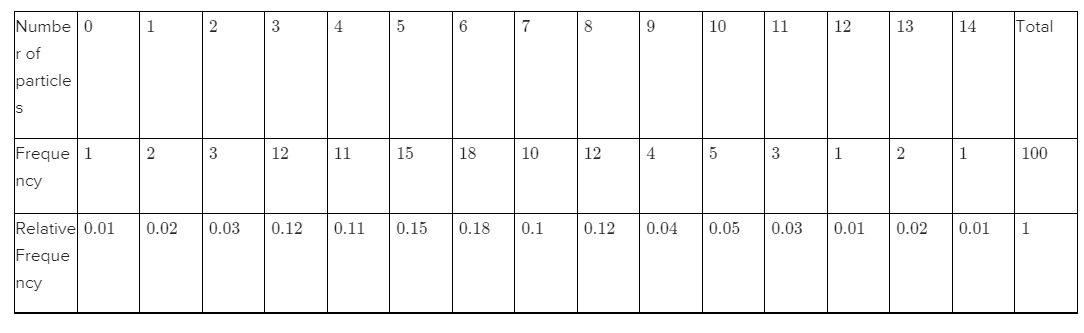
Given,Total number of sampled wafers are100.
Frequency distribution of these 100 sampled wafers i.e.,
We need to find the proportion of the sampled wafers that had at least one particle.
Then find the proportion of the sampled wafers that had at least five particles.
Let us determine the proportion of the sampled wafers that had at least one particle.
In the given frequency distribution,Total number of sampled wafers are100.
Now, there is only first sampled wafer i.e., “0”, which does not have any particle.
Thus, the number of sampled wafers that had at least one particle are(100−1).
ORthe number of sampled wafers that had at least one particle are: 2+3+12+11+15+18+10+12+4+5+3+1+2+1=99
Therefore, proportion of the sampled wafers that had at least one particle is given by:
p= number of sampled wafers that had at least one particle
Total number of sampled wafers
This implies, p=99%
Let us determine the proportion of the sampled wafers that had at least five particles.
In the given frequency distribution,Total number of sampled wafers are 100.
Number of sampled wafers that had less than 5 particles are:100−(11+12+3+2+1)=71
OR the number of sampled wafers that had at least five particles are: 15+18+10+12+4+5+3+1+2+1=71
Therefore, proportion of the sampled wafers that had at least five particles is given by:
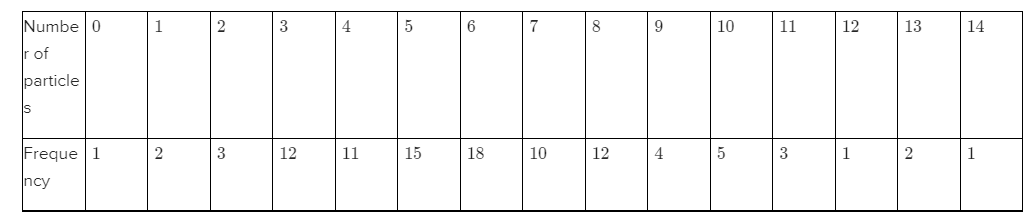
p= number of sampled wafers that had at least five particles
Total number of sampled wafers
p=71/100
p=0.71
This implies, p=71%
Therefore,the proportion of the sampled wafers that had at least one particle is 0.99=99 %.
Proportion of the sampled wafers that had at least five particles is 0.71=71%
Chapter 1 Exercise 1.2 Probability And Statistics Study Guide Page 25 Problem 11 Answer
Given, Total number of sampled wafers are 100.
Frequency distribution of these 100 sampled wafers i.e.,
we need to find the proportion of the sampled wafers having particles between five and ten, inclusive.
Then we have to find proportion of the sampled wafers having particles strictly between five and ten.
We need to find out the proportion of the sampled wafers having particles between five and ten, inclusive
That is, we need to find out the proportion of the sampled wafers having particles between five and ten, including 5 and 10.
It is given that total number of sampled wafers are 100.
Number of sampled wafers having particles between five and ten, including 5 and 10.
15+18+10+12+4+5=64 Using proportion formula, The proportion of the sampled wafers having particles between five and ten, inclusive is: p= number of sampled wafers having particles between 5 and 10 , inclusive total number of sampled wafers
p=64/100
p=0.64
This implies, p=64%
We need to find out the proportion of the sampled wafers having particles strictly between five and ten.
That is, we need to find out the proportion of the sampled wafers having particles between five and ten, not including 5 and 10.
It is given that total number of sampled wafers is 100.
Number of sampled wafers having particles strictly between five and ten are: 18+10+12+4=44
Using proportion formula,
The proportion of the sampled wafers having particles strictly between five and ten is:
p= number of sampled wafers having particles strictly between 5 and 10
total number of sampled wafers
p=44/100
p=0.44
This implies, 44% .
Hence,from the above the proportion of the sampled wafers having particles between five and ten, inclusive is 0.64=64%.and the proportion of the sampled wafers having particles strictly between five and ten is 0.44=44%.
Page 25 Problem 12 Answer
Given:,frequency distribution of 100 sampled wafers.
We need to draw a histogram taking relative frequency on the vertical axis and number of particles on horizontal axis.
Since, it is given that total sample size is 100.
Therefore, relative frequency is obtained by dividing each frequency with100.
We need to draw a histogram of this frequency distribution such that the height of the bars are equal to the relative frequency and width of all bars is equal.
Now, the required histogram with relative frequencies on y−axis is:
In this histogram, we observed that It is not perfectly symmetric, that means it is almost symmetrical.
It has only one hump, that means it is unimodal.
There are more data points on the left side, that means it is slightly positively skewed.
Therefore, we constructed a histogram using relative frequency on the vertical axis and described the shape of the histogram.
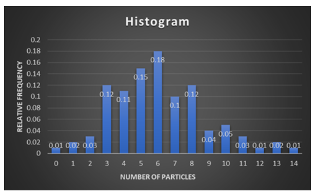
It is not perfectly symmetric, that means it is almost symmetrical.
It has only one hump, that means it is uni-modal.
There are more data points on the left side, that means it is slightly positively skewed.
Exercise 1.2 Examples From Probability And Statistics For Engineering Page 26 Problem 13 Answer
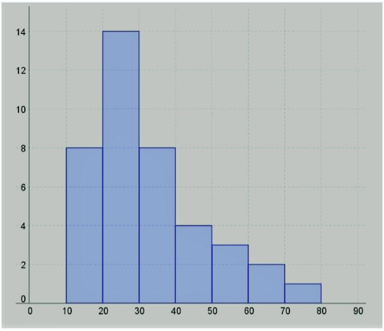
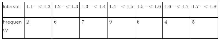
Given, An important characteristic of such an individual cell is its inter-division time representative IDT data:
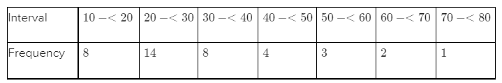
To construct a histogram of the original data using class intervals 10−<20,20−<30,…
To construct a histogram for the transformed data using the interval1.1−<1.2,1.2−<1.3,…
To describe the effect of the transformation.
In a histogram, width of the bars should be equal and height should be equal to the frequency.
To draw the histogram for the original data, we consider the following table:
Therefore, the required histogram is:
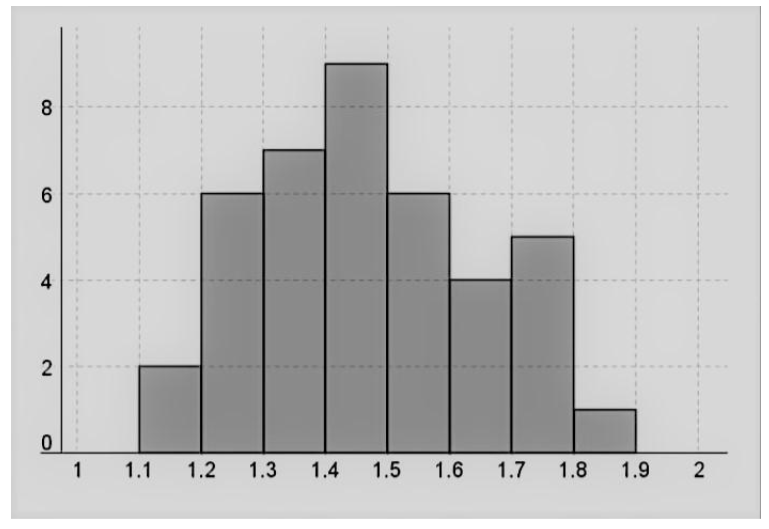
To draw the histogram for the transformed data, we consider the following table:
Therefore, the required histogram is:

The frequency distribution histogram of the original data is positively skewed as there are more data points on the left side and the highest bar is on the left side.
The frequency distribution histogram of the transformed data is slightly symmetric as there are more data points in the center and the highest bar is in the center.
Thus, we can conclude that the transformation made the distribution of the given data set more symmetric.
So,we have constructed the histogram for original and transformed data.
The transformation made the distribution of the given data set more symmetric.
Page 27 Problem 14 Answer
The given data:
⇒ 11 59 81 105 161
⇒ 14 61 84 105 168
⇒ 20 65 85 112 184
⇒ 23 67 89 118 206
⇒ 31 68 91 123 248
⇒ 36 71 93 136 263
⇒ 39 74 96 139 289
⇒ 44 76 99 141 322
⇒ 47 78 101 148 388
⇒ 50 79 104 158 513
We need to tell why can a frequency distribution not be based on the class intervals 0−50,50−100,100−150 and so on.
If suppose, we classify the distribution based on class intervals0−50,50−100 and so on, then just by looking, we would not tell that in which interval the end term in located like for example we can not tell that in which interval 50 is located, either 0−50 or 50−100.
Hence,we cannot classify the given data into class intervals due to overlapping issue.
Page 27 Problem 15 Answer
Given data,
⇒ 11 59 81 105 161
⇒ 14 61 84 105 168
⇒ 20 65 85 112 184
⇒ 23 67 89 118 206
⇒ 31 68 91 123 248
⇒ 36 71 93 136 263
⇒ 39 74 96 139 289
⇒ 44 76 99 141 322
⇒ 47 78 101 148 388
⇒ 50 79 104 158 513
We need to construct the frequency distribution and histogram.

We will construct the frequency distribution table as follows:
We have found the relative frequency by the frequency of particular interval divided by the total frequency.
The histogram is positively skewed.
It has representative value around 150. It is unimodal.
Hence,the required histogram of the data using class boundaries 0,50,100,…,is
Overview And Descriptive Statistics Notes Chapter 1 Exercise 1.2 Page 27 Problem 16 Answer
Given data is
⇒ 11 59 81 105 161
⇒ 14 61 84 105 168
⇒ 20 65 85 112 184
⇒ 23 67 89 118 206
⇒ 31 68 91 123 248
⇒ 36 71 93 136 263
⇒ 39 74 96 139 289
⇒ 44 76 99 141 322
⇒ 47 78 101 148 388
⇒ 50 79 104 158 513
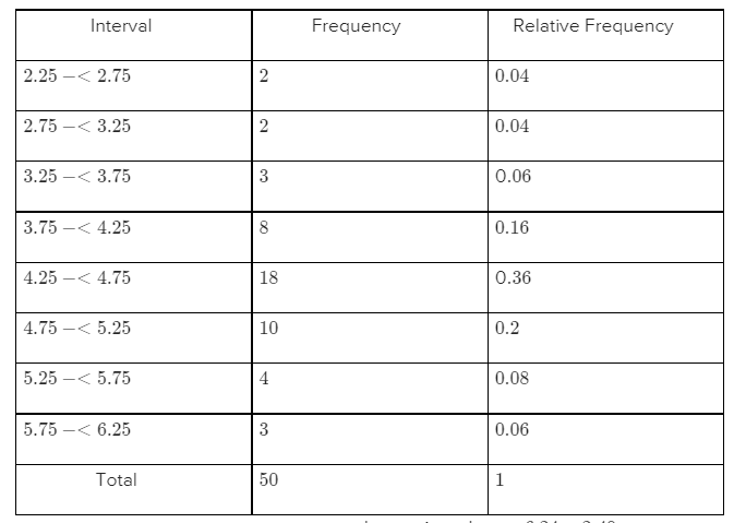
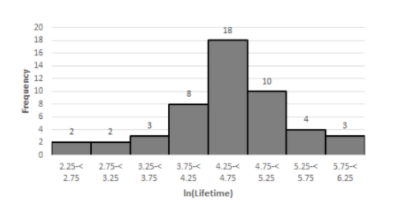
We need to construct a frequency distribution and histogram of the natural logarithms of the lifetime observations.
We will firstly determine the natural logarithm of each data point.
⇒ 2.40 4.08 4.39 4.65 5.08
⇒ 2.64 4.11 4.43 4.65 5.12
⇒ 3.00 4.17 4.44 4.72 5.21
⇒ 3.14 4.20 4.49 4.77 5.33
⇒ 3.43 4.22 4.51 4.81 5.51
⇒ 3.58 4.26 4.53 4.91 5.57
⇒ 3.66 4.30 4.56 4.93 5.67
⇒ 3.78 4.33 4.60 4.95 5.77
⇒ 3.85 4.36 4.62 5.005.96
⇒ 3.91 4.37 4.64 5.06 6.24
Now we will construct the frequency distribution:
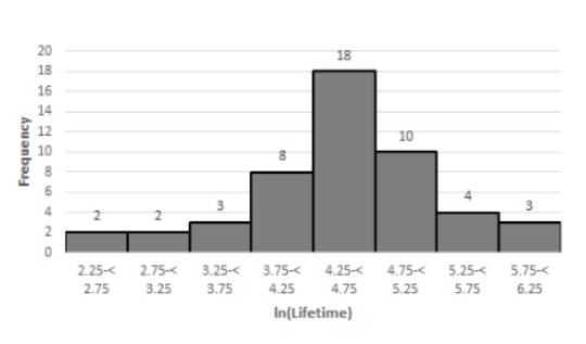
The approximate interval length = max value − min. value
√n=6.24−2.40/√50≈0.55
Since, it is not strict, we take0.5 and start from 6.25and using these we can calculate the number of intervals and their lengths.
The histogram of the given data will be
This histogram is more symmetrical than the histogram formed by the original values.
The representative value is nearly 4.5.It is unimodal.
The histogram for the log of the terms of the data is given by
This histogram is more symmetrical than the histogram formed by the original values.
The representative value is nearly 4.5.It is unimodal.
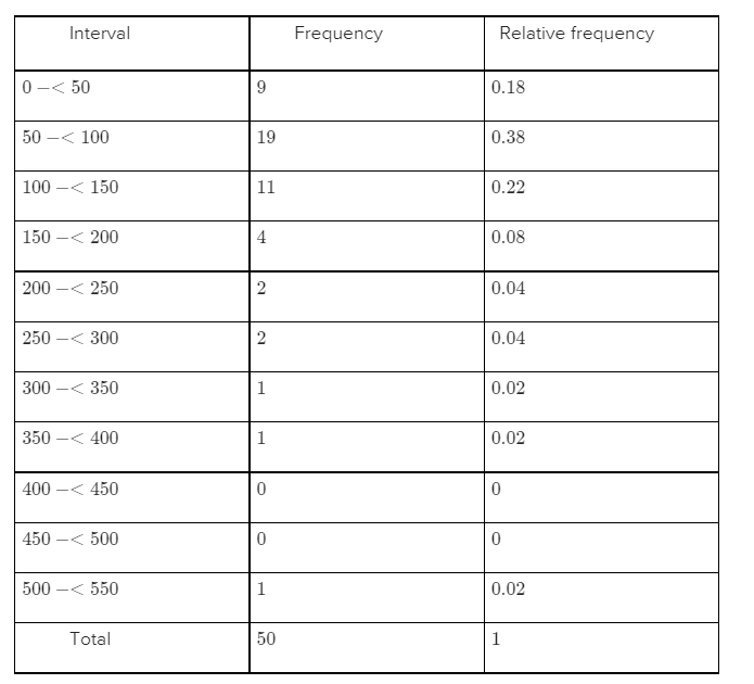
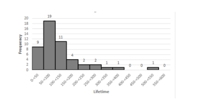
Page 27 Problem 17 Answer
According to the question, we need to find the proportion of the lifetime observations in this sample are less than 100 and proportion of the observations are at least 200 from the data:11
⇒ 59 81 105 161
⇒ 14 61 84 105
⇒ 168 20 65 85
⇒ 112 184 23 67
⇒ 89 118 206 31
⇒ 68 91 123 248
⇒ 36 71 93 136
⇒ 263 39 74 96
⇒ 139 289 44 158
⇒ 76 99 141 322
⇒ 47 78 101 148
⇒ 388 50 79 104
For the portion of the data less than 100 , we will sum up all the relative frequencies of the desired intervals.
We get 0.18+0.38=0.56 which is nearly56% .
Similarly, for the portion of the data which is at least 200,we will sum up all the relative frequencies of the desired intervals.
We get0.04+0.04+0.02+0.02+0.02=0.14 which is nearly 14%.
Hence,the portion of data which is less than 100 is 56%.
The portion of data which is at least200 is 14%.
Page 27 Problem 18 Answer
Given, Human measurements provide a rich area of application for statistical methods.
Based on the article “A Longitudinal Study of the Development of Elementary School Children’s Private Speech” reported on a study of children talking to themselves.
It was thought that private speech would be related to IQ, because IQ is supposed to measure mental maturity, and it was known that private speech decreases as students progress through the primary grades.
The study included 33
students whose first-grade IQ scores are given here:
We need to explain the data and comment on any interesting features .
Now, By plotting the given data by using Box plot then:
From the above we can observe that the data is quite large and there is positive skew.
The smallest value is 82 is separated from the remaining big sample data and can be considered outlier.
So,by plotting the given data using box plot the data is quite large and there is positive skew.
The smallest value is 82 is separated from the bulk of data so it can be considered outlier.
Study Materials For Chapter 1 Exercise 1.2 Probability And Statistics Page 27 Problem 19 Answer
Given, Consider the following data on types of health complaint made by tree planters.
The data is consistent with percentages given in the article “Physiological Effects of Work Stress and Pesticide Exposure in Tree Planting by British Columbia Silviculture Workers,” Ergonomics.
Obtain frequencies and relative frequencies for the various categories,
We need to draw a histogram.
Now, By tabulating the frequency and relative frequency of occurrence of health complaints from the given data:
| Complaint | Frequency | Relative Frequency |
| B | 7 | 0.1167 |
| C | 3 | 0.05 |
| F | 9 | 0.15 |
| J | 10 | 0.1667 |
| M | 4 | 0.0667 |
| N | 6 | 0.1 |
| O | 21 | 0.35 |
To obtain relative frequency divide by total number of observations 60.
By constructing histogram using the data:
| Complaint | Frequency | Relative Frequency |
| B | 7 | 0.1167 |
| C | 3 | 0.05 |
| F | 9 | 0.15 |
| J | 10 | 0.1667 |
| M | 4 | 0.0667 |
| N | 6 | 0.1 |
| O | 21 | 0.35 |
So, by obtaining frequencies and relative frequencies for the various categories as follows:
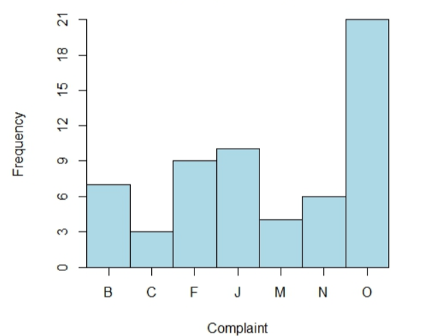
By constructing histogram using the data as follows:

Page 24 Problem 20 Answer
Given,
Failed component =126.
Incorrect component 210.
Insufficient solder =67.
Excess solder =54.
Missing component =131
From the above data, we need to construct a Pareto chart.
With the help of the given data, we will construct the Pareto diagram keeping following things in mind:
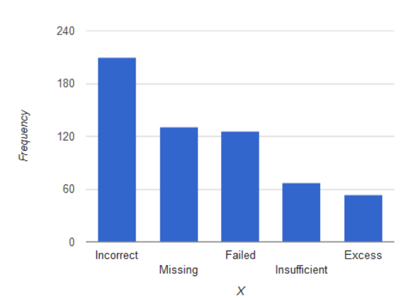
We will take equal width and the height will be equal to the frequency of the respective observation.We will rank the bars from highest to lowest.
Hence, we get Hence, the required Pareto diagram is represented on bar diagram as:

Page 27 Problem 21 Answer
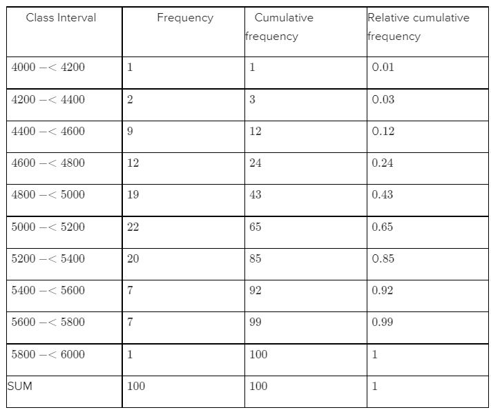
Given, According to the question, we need to compute the cumulative frequency and relative cumulative frequency of the following data:
| 5434 | 4948 | 4521 | 4570 | 4990 | 5702 | 5241 |
| 5112 | 5015 | 4659 | 4806 | 4637 | 5670 | 4381 |
| 4820 | 5043 | 4886 | 4599 | 5288 | 5299 | 4848 |
| 5378 | 5260 | 5055 | 5828 | 5218 | 4859 | 4780 |
| 5027 | 5008 | 4609 | 4772 | 5133 | 5095 | 4618 |
| 4848 | 5089 | 5518 | 5333 | 5164 | 5342 | 5069 |
| 4755 | 4925 | 5001 | 4803 | 4951 | 5679 | 5256 |
| 5207 | 5621 | 4918 | 5138 | 4786 | 4500 | 5461 |
| 5049 | 4974 | 4592 | 4173 | 5296 | 4965 | 5170 |
| 4740 | 5173 | 4568 | 5653 | 5078 | 4900 | 4968 |
| 5248 | 5245 | 4723 | 5275 | 5419 | 5205 | 4452 |
| 5227 | 5555 | 5388 | 5498 | 4681 | 5076 | 4774 |
| 4931 | 4493 | 5309 | 5582 | 4308 | 4823 | 4417 |
| 5364 | 5640 | 5069 | 5188 | 5764 | 5273 | 5042 |
| 5189 | 4986 |
Cumulative frequency of any observation can be calculated by adding up all the frequencies of previous observations.
Relative cumulative frequency of any observation= Cumulative frequency of that observation /100
We know that frequency is defined as the number of times a value occurs in the given data.
The frequency, cumulative frequency, relative cumulative frequency of the given data are given below:

Hence,we have calculated the cumulative frequency and relative cumulative frequency of every value in the data with the help of definitions as follows: