
Probability and Statistics for Engineering and the Sciences 8th Edition Chapter 1 Overview and Descriptive Statistics
Page 46 Problem 1 Answer
Given,Based on the paper “Correlation Analysis of Stenotic Aortic Valve Flow Patterns Using Phase Contrast MRI”gave the following data on aortic root diameter (cm) and gender for a sample of patients having various degrees of aortic stenosis:
Data on aortic root diameter (cm) and gender for a sample of patients
We need to compare and contrast the diameter observations for the two genders.
Initially we need to find various parameters and then make a boxplot in order to compare the data given.
The sample means. xM
xF=3.1+3.4+3.4+3.4+3.5+3.6+3.7+3.7+3.8+3.8+3.9+4.0+4.0/13
xF=3.6385
xF=2.6+3.0+3.0+3.1+3.1+3.2+3.2+3.5+3.8+4.3/10
xF=3.28
We can observe that the sample mean is greater for males than for females.
Standard deviation for both samples.
sM=√1/13−1[(3.1−3.6385)2+(3.4−3.6385)2+⋅(3.4−3.6385)2+(3.4−3.6385)2+(3.5−3.6385)2+(3.6−3.6385)2+(3.7−3.6385)2+(3.7−3.6385)2+(3.8−3.6385)2+]
(3.8−3.6385)2+(3.9−3.6385)2+(4.0−3.6385)2+(4.0−3.63)+85)2]
sM=0.2694
sF=√1/10−1[(2.6−3.28)2+(3.0−3.28)2+(3.0−3.28)2+(3.1−3.28)2+(3.1−3.28)2+(3.2−3.28)2+(3.2−3.28)2+(3.5−3.28)2+(3.8−3.28)2+(4.3−3.28)2]=0.4780
We can observe that the sample standard deviation is greater for females than for males.
Arranging each sample in the increasing order-
M:{3.1,3.4,3.4,3.4,3.5,3.6,3.7,3.7,3.8,3.8,3.9,4.0,4.0}
F:{2.6,3.0,3.0,3.1,3.1,3.2,3.2,3.5,3.8,4.3}
For a box-plot we need-The median is given by the element for males and by the average of the for females.
xM/N=3.7
xF=3.1+3.2/2
xF=3.15 − lower fourth M
xF=3.4 ,lower fourth F
xF=3.0 − upperfourth M
xF=3.8 ,upperfourth F
xF=3.5 − fs/M
Fs/F= upper fourth M− lower fourth M
Fs/F=3.8−3.4
Fs/F=0.4
= upper fourth F− lower fourth F
=3.5−3.0
=0.5
M:smallest xi=3.1and largest xi=4.0
F:smallest xi=2.6 and largest xi=4.3
The boxplot can be constructed as-
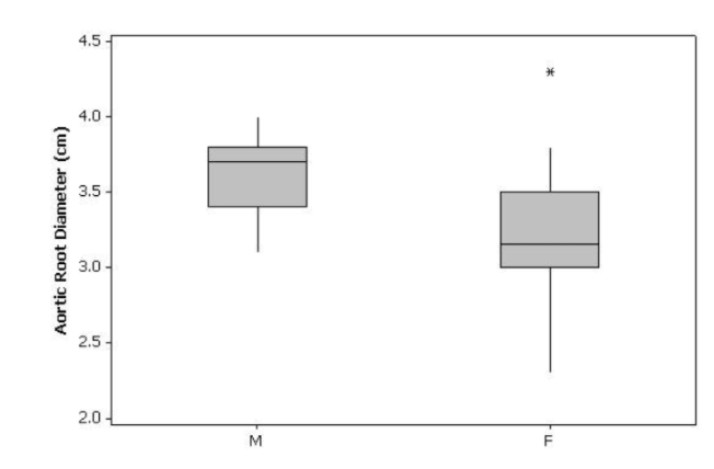
The values for the M-sample are greater than female.
The boxplot and standard deviations suggest that variability is smaller for the M-sample.
An outlier, , in the female sample exists. There is positive overall skew in the F-sample and negative skew in the M-sample.
Hence,based on the given data the mean, standard deviation, median, Q1,Q3 and fs
for M-sample are 3.6385,0.2694,3.7,3.4,3.8 and 0.4 respectively.
The mean, standard deviation, median, Q1 , Q3 and fs for F-sample are 3.28,0.4780,3.15,3.0,3.5 and 0.5 respectively.
Thus the boxplot is-
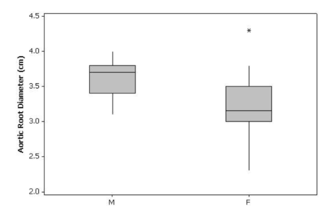
The typical values for the M-sample are greater greater than female.
The boxplot and standard deviations suggest that variability is smaller for the M-sample. An outlier, 4.3, in the female sample exists.
There is positive overall skew in the F-sample and negative skew in the M-sample.
Probability And Statistics For Engineering 8th Edition Supplementary Exercise Solutions Page 46 Problem 2 Answer
Given that aortic stenosis refers to a narrowing of the aortic valve in the heart.
The paper “Correlation Analysis of Stenotic Aortic Valve Flow Patterns Using Phase Contrast MRI” gave the following data on aortic root diameter (cm) and gender for a sample of patients having various degrees of aortic stenosis:
Data on aortic root diameter (cm) and gender for a sample of patients.
We need to find 10% trimmed mean for each of the two samples, and compare to other measures of center.
First, calculate both the trimmed means one by one.
The 10% trimmed mean for the M-sample.
So, (.1)(13)=1.3 elements need to be eliminated from each end of the sample, i.e. eliminate 1
and then elements at each end.
pU/pF=100(1/13)
pU/pF=7.692%
pU/pF=100(2/13)
pU/pF=15.385%
So now trimmed mean for xtr(7.692)M and xtr(15.385)M/
xˉ=3.4+3.4+3.5+3.6+3.7+3.7+3.8+3.8+3.9+4.0/11
xˉ=3.6545
xˉ=3.4+3.4+3.5+3.6+3.7+3.7+3.8+3.8+3.9/9
xˉ=3.6444
Interpolate between xm(7.692)M and xtr(15.385) M to find xtr(10) M.
xtr(10)Mˉ=0.7⋅xtr(7.692)M−+0.3⋅xtr(15.385)M−
xtr(10)Mˉ=(0.7)(3.6545)+(0.3)(3.6444)
xtr(10)Mˉ=3.6515
We can observe that it is greater than the actual mean of the M-sample but smaller than the median.
For, xrr(10)F eliminate (.1)(10)=1 value from each end of the ordered -sample.
xˉ=3.0+3.0+3.1+3.1+3.2+3.2+3.5+3.8/8
xˉ=3.2375
We can observe that it is smaller than the actual mean of the F-sample but greater than the median.
Therefore,based on the paper “Correlation Analysis of Stenotic Aortic Valve Flow Patterns Using Phase Contrast MRI” gave the following data on aortic root diameter (cm) and gender for a sample of patients having various degrees of aortic stenosis we get the following:
The 10% trimmed mean for M- sample and F-sample are 3.6515 and 3.2375 respectively.
We can observe that it is greater than for both M- sample and F-sample the trimmed mean is smaller than the actual mean but greater than the median.
Page 47 Problem 3 Answer
Given, Based on the article “Establishing mechanical property allowables for metals” we get:
From the given information, we get that:
The sample mean, the sample median, and the trimmed mean have almost the same values.
This shows that the data is very symmetrical and there is no presence of outliers.
If in the worst-case scenario there exists outliers then they are balanced out.
This means that the bigger value would be at the same distance from the mean as the smaller value would be.
All of the values are between122.2 and 147.7.
Variability of the data is very small.
Therefore, based on the article “Establishing mechanical property allowables for metals” the following observations: we can say that:
The data has a symmetric distribution.
There are balanced outliers present.
The range of the data is 25.5.
Page 47 Problem 4 Answer
Given, Based on the article “Establishing mechanical property allowables for metals” as follows.
From the given information, we get that:
Since we are already given the five-number summary, we need to determine whether outliers are present or not.
We distribute our outliers into two categories, extreme and mild outliers.
We need to construct boxplot based on the given data.
In this step, we will determine the fourth spread of our data:
fs=Q3−Q1
⇒138.25−132.95
⇒5.3
In this step, we will determine the limits of mild and extreme outliers along with specific values of outliers if present.:
The criteria for any data to be an outlier is that it must be further than 1.5f{s} than either Q{1} Or Q{3}.
An outlier is said to be an extreme outlier if it is further than 3f{s} than either Q{1} or Q{3} otherwise, it is said to be a mild outlier.
Since fs=5.3 : 1.5fs
fs =1.5×5.3
⇒7.95
3fs=3×5.3
⇒15.9
Then the limits for mild outliers are,
Q3+1.5fs
=138.25+7.95
⇒146.2
Q1−1.5fs
=132.95−7.95
⇒125
The limits for extreme outliers are,
Q3+3fs
=138.25+15.9
⇒154.15
Q1−3fs
=132.95−15.9
⇒117.05
Therefore we can say that mild outliers lie between [117.05,125] and [146.2,154.15]
We can also say that extreme outliers are values that are smaller than 117.05 and greater than 154.15 .
Hence there are mild outliers present in our data. These are:
117.05<122.2,124.2,124.3<125 and 147<147.7,147.7<154.15
Therefore, our lower data is 122.2,124.2,124.3,125.6,126.3 and our high data is
144.1,144.5,144.5,147.7,147.7
The box plot for the exercise prompt is:
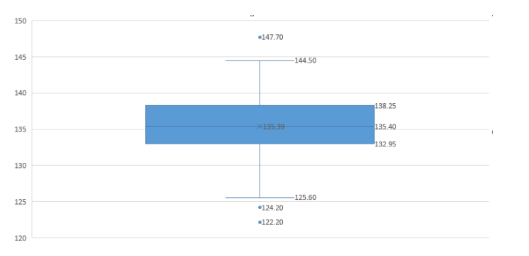
Therefore,based on the article “Establishing mechanical property allowables for metals” the following are obtained:
the final boxplot for the given statistical inference is given as:
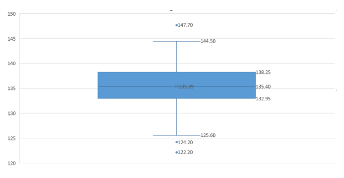
From the box plot we can see that we have 3 outliers: 122.2,124.2, and 147.7.
The median of the box-plot is 135.4.
Chapter 1 Supplementary Exercise Overview And Descriptive Statistics Page 47 Problem 5 Answer
Given, Based on the paper “Decreased Benzodiazepine Receptor Binding in Prefrontal Cortex in Combat-Related Post traumatic Stress Disorder” described the first study of benzodiazepine receptor binding in individuals suffering from PTSD the following data are given:
| Variable | N | Mean | SE Mean | TrMean | StDev | Minimum | Q1 | Median | Q3 |
| PSTD | 13 | 32.92 | 2.75 | 33.82 | 9.93 | 10 | 26.5 | 37 | 39 |
| Healthy | 13 | 52.23 | 4.12 | 53.09 | 14.86 | 23 | 40.5 | 51 | 66.5
|
| Variable | Maximum |
| PSTD | 46 |
| Healthy | 72 |
We need to use various methods from this chapter to describe and summarize the data.
Construction of box plot using MINITAB
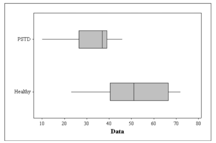
Hence,based on the paper “Decreased Benzodiazepine Receptor Binding in Prefrontal Cortex in Combat-Related Post traumatic Stress Disorder” data
the above box plot shows that PSTD has larger variance than Healthy data and also in PSTD the data distribution in left skewed whereas right skewed in Healthy data.
Page 47 Problem 6 Answer
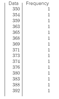
Given,Based on the article “Can We Really Walk Straight?”reported on an experiment in which each of 20 healthy men was asked to walk as straight as possible to a target 60 m away at normal speed the data as follows:
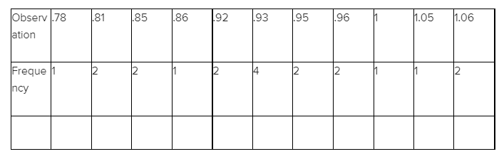
Use the methods developed in this chapter to summarize the data; include an interpretation or discussion wherever appropriate.
Count the number of observations which is repeated most often to get the mode.
Now,Frequency of observation is shown below :
Hence,based on the article “Can We Really Walk Straight?”reported on an experiment in which each of 20 healthy men was asked to walk as straight as possible to a target 60 m away at normal speed the following are obtained as:
The required mode is 0.93.
Page 47 Problem 7 Answer
Given,Based on the article “Can We Really Walk Straight?”reported on an experiment in which each of 20
healthy men was asked to walk as straight as possible to a target 60
m away at normal speed the data as follows:
We are given our dataset and we are asked to find the mode.
Since the mode is the most frequent value, we will parse through our dataset and find the data which occurs the most.
Then, resulting data is the mode for the cadence dataset.
The dataset given is, .95.85.92.95.93.861.00.92.85.81.78.93.93
⇒ 1.05.931.061.06.96.81.96
We observe that the data 0.93 occurs the most with a frequency of 4.
Therefore, the mode for the data is 0.93.
Hence,based on the article “Can We Really Walk Straight?”reported on an experiment in which each of 20 healthy men was asked to walk as straight as
possible to a target 60m away at normal speed the data as follows:
The mode for the cadence data is 0.93.
Solved Examples For Supplementary Exercise In Probability And Statistics 8th Edition Page 47 Problem 8 Answer
Given, We are given the dataset of cadence and we are asked to define the modal category for a categorical sample.
In simple terms, the category which would contain the most observations would be known as the modal category.
Therefore,for a categorical sample, we would define the modal category as follows:
The category which would contain the most observations would be known as the modal category.
Page 47 Problem 9 Answer
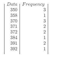
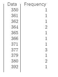
Given, Specimens of three different types of rope wire were selected, and the fatigue limit (MPa) was determined for each specimen, resulting in the accompanying data as follows:
The five number summary of three different types of ropes are
We need to construct a comparative boxplot, and comment on similarities and differences.
The box plot of three different type of ropes is :
| 350 | 358.00 | 371.00 | 384.00 | 392.00 |
| 350 | 363 | 371 | 380 | 392 |
| 350 | 364 | 370 | 379 | 392 |
Since the distributions have same minimum and maximum value i.e.350 and 392 respectively, all the three have symmetric distribution.
But the first and fourth quadrant values are different.
Hence, we can conclude that Type1 is more spread out than the other two, therefore the data is more dispersed in Type1 with largest inter quartile range.
Page 47 Problem 10 Answer
Given,Specimens of three different types of rope wire were selected, and the fatigue limit (MPa) was determined for each specimen, resulting in the accompanying data as follows:
In order to plot the dot-plot for all the three different types of ropes, we will find the count for the data values in the data set.
We need to construct a comparative dot plot (a dot plot for each sample with a common scale) and comment on similarities and differences.
For type1 sample:
Therefore, the dot-plot for the following datasets are:
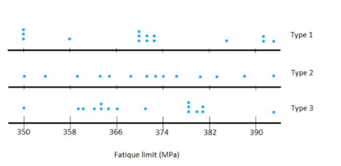
Hence,based on the given data the dot-plot for the dataset can be as as follows:
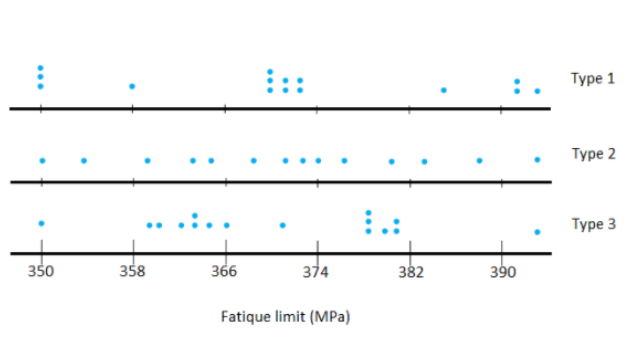
Page 47 Problem 11 Answer
Given, Specimens of three different types of rope wire were selected, and the fatigue limit (MPa) was determined for each specimen, resulting in the accompanying data:
In order to create a box-plot we need five numbers that will summarize the data.
They are:
1) smallest xi
2)lower fourth,
3)Median,
4)upper fourth,
5)largest xi
Therefore, the boxplot does not give an informative assessment of similarities and differences.
In this case, the dot plot explained the dataset in a more enhanced way.
Therefore the boxplot is not able to give an informative assessment of similarities and differences.
Probability And Statistics 8th Edition Chapter 1 Supplementary Exercise Page 48 Problem 12 Answer
Given,Based on the authors of the article “Predictive Model for Pitting Corrosion in Buried Oil and Gas Pipelines” (Corrosion, 2009: 332–342) provided the data on which their investigation was based as follows:
To make the Steam-and-Leaf Display:
| Stem | Leaves |
| 0L | 414141414343434000 |
| 0H | 587979818181919000 |
| 1L | 2.04E+24 |
| 1H | 4040 |
| 2L | 5959606891969690 |
| 2H | 1021314649 |
| 3L | 5774 |
| 3H | 101830 |
| 4L | 5858 |
| 4H | 15 |
| 5L | 75 |
| 5H | 33 |
| 6L | 6570 |
| 6H | 13 |
| 7L | HI: 10.41,13.44 |
| 7H | |
| 8L |
We need to construct a stem-and-leaf display in which the two largest values are shown in a last row labeled HI.
Select the leading digits, following that, the digits coming after the leading digits are the leaves.
Then list the values of the stem we obtained in a column.
Note down the leaf for all data values associated with the particular stem value.
Finally, note down the units of the stem and leaves.
The leading digits (ones) for the data in the exercise are:
0,1,2,3,4,5,6,7,8
Listing the leading digits we get:
Stem
0
1
2
3
4
5
6
7
8
Let us denote:L (lower): the tenth digits which are less than 5.H (higher): the tenth digits which are more than or equal to 5.
We then have our stem to be:
Stem
0L
0H
1L
1H
2L
2H
3L
3H
4L
4H
5L
5H
6L
6H
7L
7H
8L
Recording the leaves for each and every observation and obtain the Stem-and-leaf display:
| Stem | Leaves |
| 0L | 414141414343434000 |
| 0H | 587979818181919000 |
| 1L | 2.04E+24 |
| 4040 | |
| 1H | 5959606891969690 |
| 2L | 1021314649 |
| 2H | 5774 |
| 3L | 101830 |
| 3H | 5858 |
| 4L | 15 |
| 4H | 75 |
| 5L | 33 |
| 5H | |
| 6L | |
| 6H | |
| 7L | |
| 7H | 6570 |
| 8L | 13 HI: 10.41,13.44 |
Hence ,based on the authors of the article “Predictive Model for Pitting Corrosion in Buried Oil and Gas Pipelines” provided the data on which their investigation was based obtained as follows:
The stem-and-leaf display is given as:
| Stem | Leaves |
| 0L | 414141414343434000 |
| 0H | 587979818181919000 |
| 1L | 2.04E+24 |
| 4040 | |
| 1H | 5959606891969690 |
| 2L | 1021314649 |
| 2H | 5774 |
| 3L | 101830 |
| 3H | 5858 |
| 4L | 15 |
| 4H | 75 |
| 5L | 33 |
| 5H | |
| 6L | |
| 6H | |
| 7L | |
| 7H | 6570 |
| 8L | 13 HI: 10.41,13.44 |
Chapter 1 Supplementary Exercise Study Guide In Probability And Statistics Page 48 Problem 13 Answer
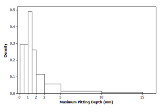
Given,The authors of the article “Predictive Model for Pitting Corrosion in Buried Oil and Gas Pipelines”provided the data on which their investigation was based as follows:
As the given classes have different widths,
we should construct a density histogram make a table having class, frequency, relative frequency, density.
The formula for relative frequency for each class can be defined as the ratio of the frequency to the total number of observations.
As the given classes are having different widths so, we have to construct a density histogram.
For each class the density is given by the formula: rectangle height = relative frequency of the class/class width
Table is described below:-
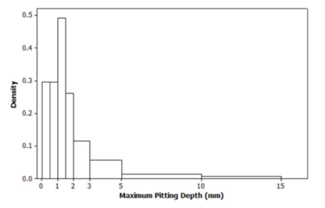
After getting the desired values, the graph is constructed as
Hence,based on the authors of the article “Predictive Model for Pitting Corrosion in Buried Oil and Gas Pipelines” (Corrosion, 2009: 332–342) provided the data on which their investigation was based:
A histogram graph is shown below
Page 48 Problem 14 Answer
Given, Based on the authors of the article “Predictive Model for Pitting Corrosion in Buried Oil and Gas Pipelines” (Corrosion, 2009: 332–342) provided the data on which their investigation as follows:
By observing the comparative boxplot for different types of soils:
For all types of soil, values are quite similar:
The largest variability holders are in C and CL types.
For SYCL type of soil, there is mild positive overall skew.
significant positive overall skew is shown by the first three types i.e.(C,CL,SCL).
While negative skew id presented by the middle of the data.
For the first three types of soils include extreme one The values for all types of soil are almost same as they are represented in the graph.
Some show positive overall skew while some show mild positive overall skew.
Hence, Important features are described as below.
For all types of soil, values are quite similarThe largest variability holders are in C and CL types.
For SYCL type of soil, there is mild positive overall skew.significant positive overall skew is shown by the first three types i.e.(C,CL,SCL).
While negative skew id presented by the middle 50% of the data.
For the first three types of soils include extreme one
Page 48 Problem 15 Answer
Given,The article “Planning of City Bus Routes”gives the following information on lengths (km) for one particular system:
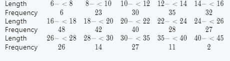
We need to draw a histogram for the above given data.
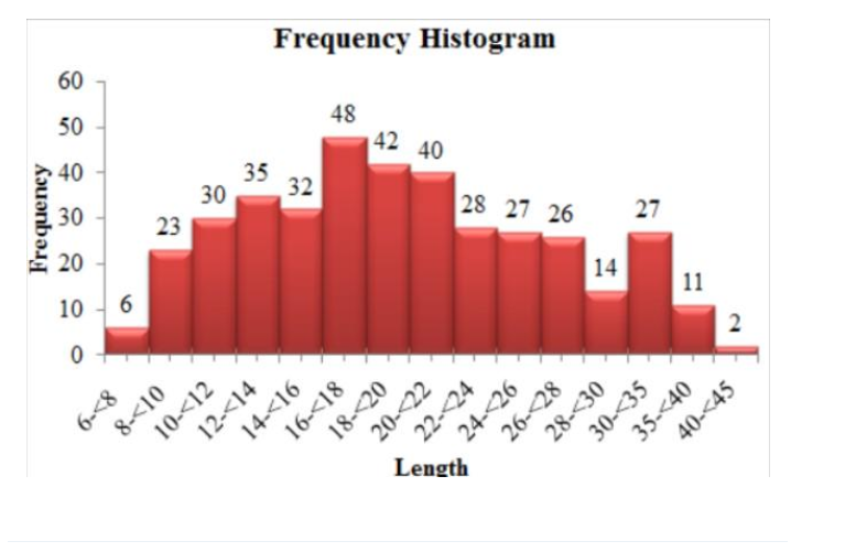
Hence,according to length and frequencies, histogram is drawn shown below:

Examples From Supplementary Exercise In Probability And Statistics For Engineering Page 48 Problem 16 Answer
Given, The article “Planning of City Bus Routes”gives the following information on lengths (km) for one particular system: number which is less then 20:-6,23,30,35,32,48,42
Given number which is at least 30:- 27,11,2
N= some of all frequency that is 391 Less than 20=6+23+30+35+32+48+42/N
N=6+23+30+35+32+48+42/391
N=216/391
N=0.5524
Therefore, the proportion of route lengths are less than 20 is 0.5524.
atleast 30=27+11+2/N
=40/391
=0.1023
Therefore, the proportion of routes have lengths of at least 30 is0.1023.
Therefore, the proportion of route lengths are less than 20 is 0.5524 .
Therefore, the proportion of routes have lengths of at least 30 is 0.1023 .
Page 48 Problem 17 Answer
Given,Based on the article “Planning of City Bus Routes” gives the following information on lengths (km) for one particular system:
The cumulative frequency table is,
| Class | 0−<0.5 | 0.14754 | 0.4918 | 0.2623 |
| Frequency | 9 | 4 | 2 | |
| Relative | 0.14754 | 0.29508 | 0.06557 | 0.03279 |
| Frequency | 7 | 0.01311 | 0.00656 | |
| Density | 0.29508 | 0.11475 | 1.5−2 | |
| Frequency | 7 | 0.05738 | 8 | |
| Relative Frequency | 0.11475 | 1−<1.5 | 0.13115 | |
| 0.11475 | 15 | |||
| Density | 0.5−1 | 0.2459 | ||
| 9 |
Here , N=391
90th position is 90N
100=351.9
The cumulative frequency just greater than 351.9 is 378 . The corresponding class is 30−35 . The lower limit of the class is 30 . The corresponding frequency is 27.
Use the following formula to compute the 90th percentile,P∞=I+h/f (90N/100−C)
Here, l is the lower limit of the median class = 30,
h is the height of the median class= 5.
C is the prior cumulative of frequency of the median class = 351
On substituting the values in the above formula:
P90=30+5/27(90(391)/100−351)
P90=30+5/27(351.9−351)
P90=30.1667
Therefore, the 90th percentile is 30
Hence,based on the article “Planning of City Bus Routes” (J. of the Institution of Engineers, 1995: 211–215) gives the following information on lengths (km) for one particular system obtained as follows:
Therefore, the 90th percentile is 30.
Page 48 Problem 18 Answer
Given, Lengths of bus routes for any particular transit system will typically vary from one route to another.
Based on the article “Planning of City Bus Routes”gives the following information on lengths (km) for one particular system:
l=18,
h=2,
f=42,
C=174
We need to find the median route length.
Compute the median route length.
N/2=(391)/2
N/2 =195.5
The cumulative frequency (c.f) just greater than 195.5 is 216. Median =l+h/f(N/2−C) on substituting, Median
=18+2/42(195.5−174)
=18+(0.0476)(21.5)
=18+1.0238
=19.0238
Therefore, the median route length is 19.0238
Hence,based on the article “Planning of City Bus Routes”gives the following information on lengths (km) for one particular system: the median route length is 19.0238.
Notes For Supplementary Exercise Overview And Descriptive Statistics Chapter 1 Page 49 Problem 19 Answer
Given,Consider the following time series in which x{t}=temperature in Fahrenheit of effluent at a sewage treatment plant on day t: 47,54,53,50,46,46,47,50,51,50,46,52,50,50
We need to plot xtˉagainst t on a two-dimensional coordinate system (a time-series plot) and does there appear any pattern.
Now, Consider the times series of effluent at a sewage treatment plant on day t:
The data set has a range of values from 46 to 54.
By plotting the data points on temperature time series plot we get:
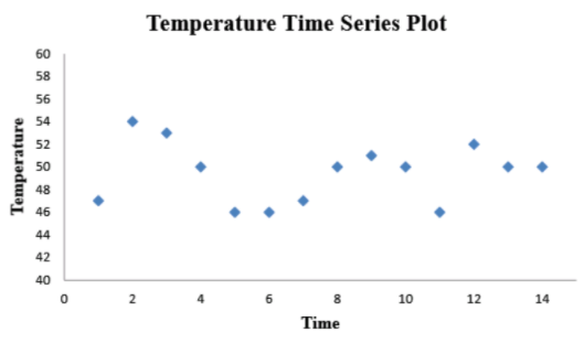
By observing the time series plot the data appears to be cyclical pattern similar to the sine wave.
So,by plotting the temperature time series data points we get :

By observing the time series plot the data appears to be cyclical pattern similar to the sine wave.
Page 49 Problem 20 Answer
Given, Smoothing constant: forα=.1
Initially set X1ˉ=x1
forα=.5
We need to calculate the xtˉ
| t | x |
| 1 | 47 |
| 2 | 47.7 |
| 3 | 48.23 |
| 4 | 48.41 |
| 5 | 48.17 |
| 6 | 47.95 |
| 7 | 47.85 |
| 8 | 48.07 |
| 9 | 48.36 |
| 10 | 48.53 |
| 11 | 48.27 |
| 12 | 48.65 |
| 13 | 48.78 |
| 14 | 48.9 |
for different values of smoothing constant given above.
Then we need to comment that for which value of α the xtˉseries is smoother.
x2ˉ=α⋅x2+(1−α)⋅x1ˉ=(0.1)(54)+(1−0.1)(47)
=47.7 and thren use the same method to compute, x3ˉ
x3ˉ=α⋅x3+(1−α)⋅x2ˉ=(0.1)(53)+(1−0.1)(47.7)=48.23
Now repeat this process to get a table for all values in the time series dataset, with α=0.1
Repeat the exponential smoothing technique with α=0.5 to obtain the another table of data,.
| t | x |
| 1 | 47 |
| 2 | 50.5 |
| 3 | 51.75 |
| 4 | 50.88 |
| 5 | 48.44 |
| 6 | 47.22 |
| 7 | 47.11 |
| 8 | 48.55 |
| 9 | 49.78 |
| 10 | 49.89 |
| 11 | 47.94 |
| 12 | 49.97 |
| 13 | 49.99 |
| 14 | 49.99 |
The process is exactly the same as before, only with a different value of α Exponential Smoothing with α=0.5
The first series withα=0.1 seems to be smoother than the second series with α=0.5.
The first series is smoother because there is less variability between values .
Additionally, the first series switches between increasing and decreasing less frequency.
When the first series does switch between increasing and decreasing, the magnitude the switch is much less than that of the switches in the second series.
Therefore, after examining both series, α=0.1 yields a smoother series
Study Materials For Supplementary Exercise In Chapter 1 Probability And Statistics Page 49 Problem 21 Answer
Given,Substituting Xt−1−=αXt−1 +(1−α)Xt−2−on the right-hand side of the expression forxˉ,then substitute Xt−2−in terms of Xt−2 and Xt−3−,
We need to find the number of values xt,xt−1,…,x1 does xˉ depend and what happens to the coefficient xt−k on as k increases.
Perform the substitution as directed in the problem statement.
xtˉ=α⋅xt+(1−α)⋅xt−1−=α⋅xt+(1−α)⋅[α⋅xt−1+(1−α)⋅xt−2−]
xtˉ =α⋅xt+α⋅(1−α)⋅xt−1+(1−α)2⋅xt−2−
Repeat the process again and substitute x in terms of x and x . t−2−t−2 t−3−
xt = α ⋅ xt + α ⋅ (1 − α) ⋅ xt−1 + (1 − α) ⋅ x/2t−2−
xt = α ⋅ xt + α ⋅ (1 − α) ⋅ xt−1 + (1 − α) ⋅ α ⋅ x + (1 − α) ⋅ x2[ t−2 t−3−]
xt = α ⋅ xt + α ⋅ (1 − α) ⋅ xt−1 + α ⋅ (1 − α) ⋅ x + (1 − α) ⋅ x2t−2/3t−3−
xt = (1 − α) ⋅ x + α ⋅ (1 − α) ⋅ x3/t−3− ∑k=0 2 ki−k
repeat this process, and recalling that xˉ = x1, using the following formula From
xˉt = (1 − α) ⋅ + α ⋅ (1 − α) ⋅ x t−1 xˉ1 ∑k=0 t−2 k t−k
xˉt = (1 − α) ⋅ x + α ⋅ (1 − α) ⋅ x t−1 1 ∑k=0 t−2 k t−k
the formula, depends on all of the previous values This is true because each value appears in the formula for so each value has an impact on the value of .
Thus depends on all of the previous values
xˉt
xˉt xt, xt−1,…, x1
Since is between zero and one, is between zero and one, so raising it to higher and higher powers causes the value to get smaller.
This is precisely what happens to the coefficient of as the value of k increases.
In the limit, this coefficient goes to zero as k goes to infinity.
Thus, as k increases the coefficient of decreases
So,xtˉ depends on all of the previous values xt,xt−1,…,x1 which aret−1 terms.
As k increases the coefficient of xt−k decreases.
Page 49 Problem 22 Answer
Given,The sample data X1,X2,…,Xn represents a time series.
X1ˉ=x1
If t is large, we need to find how sensitive is Xtˉ to the initialization X1ˉ=x1 and explain.
Since, a is between zero and one, 1−α is between zero and one, so raising it to higher and higher powers causes the value to get smaller.
This is precisely what happens to the coefficient of xt−k as the value of k increases.
In the limit, this coefficient goes to zero as k goes to infinity.
Therefore,it is proved that xtˉ is very insensitive to the initialization x1ˉ=x1.